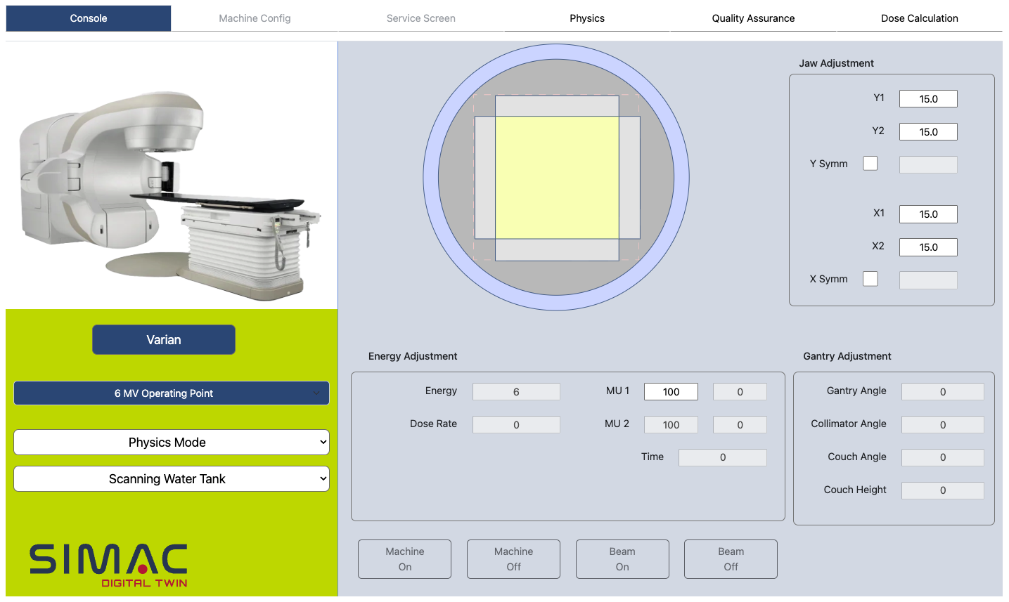
The Console is where every session begins. Pick the machine, load an operating point, choose a mode and turn the beam on. From here you branch to: 1. Machine Config — the per-subsystem tabs where you build and tune a beam. 2. Service Screen – the service screen emulator that mimics that controls in Machine Config. 3. Physics – which holds the two virtual water tanks for scanning and calibrating the beams you saved. 4. Quality Assurance – where you can upload your real QA data. 5. Dose Calculation – the interface to run a dose calibration on the beams you saved.
1
2
3
4
5
6
7
8
9
Numbered markers match the list below.
What each area does
1
Application tabs
Console, Service Screen, Machine Config, Physics, Quality Assurance, and Dose Calculation.
2
Machine select
Select Varian or Elekta. This sets which simulator model — and therefore which tab layout — you operate.
3
Operating point
Choose a default energy (e.g. 6 MV Operating Point) or a previously saved beam.
4
Operation mode
Machine Config, Service Mode or Physics Mode. Machine Config opens the subsystem tabs in this manual; Physics Mode reveals the water-tank selector below.
5
Water-tank selector
Shown in Physics Mode. Pick Scanning Water Tank (profiles & PDD) or Calibrating Water Tank (mock TG51 / TRS-398).
6
Jaw Adjustment
Set X1 / X2 and Y1 / Y2 (with optional symmetry lock). The field is reflected live in the central beam's-eye view.
7
Energy / MU / Time
Set MU1 and MU2 for the length of the beam; read back Energy, Dose Rate and Time.
8
Gantry Adjustment
Gantry, collimator and couch angles plus couch height. Not set up in the current build.
9
Machine & beam controls
Machine On / Off and Beam On / Off — another place to control the simulation, mirroring the controls inside Machine Config.
See also
Overview
Perform a scan
Calibration (TG51 / TRS-398)
Getting started
The Console — your starting point
CONSOLE
The Console is where every session begins. Pick the machine, load an operating point, choose a mode and turn the beam on. From here you branch to: 1. Machine Config — the per-subsystem tabs where you build and tune a beam. 2. Service Screen – the service screen emulator that mimics that controls in Machine Config. 3. Physics – which holds the two virtual water tanks for scanning and calibrating the beams you saved. 4. Quality Assurance – where you can upload your real QA data. 5. Dose Calculation – the interface to run a dose calibration on the beams you saved.
1
2
3
4
5
6
7
8
9
Numbered markers match the list below.
What each area does
1
Application tabs
Console, Service Screen, Machine Config, Physics, Quality Assurance, and Dose Calculation.
2
Machine select
Select Varian or Elekta. This sets which simulator model — and therefore which tab layout — you operate.
3
Operating point
Choose a default energy (e.g. 6 MV Operating Point) or a previously saved beam.
4
Operation mode
Machine Config, Service Mode or Physics Mode. Machine Config opens the subsystem tabs in this manual; Physics Mode reveals the water-tank selector below.
5
Water-tank selector
Shown in Physics Mode. Pick Scanning Water Tank (profiles & PDD) or Calibrating Water Tank (mock TG51 / TRS-398).
6
Jaw Adjustment
Set X1 / X2 and Y1 / Y2 (with optional symmetry lock). The field is reflected live in the central beam's-eye view.
7
Energy / MU / Time
Set MU1 and MU2 for the length of the beam; read back Energy, Dose Rate and Time.
8
Gantry Adjustment
Gantry, collimator and couch angles plus couch height. Not set up in the current build.
9
Machine & beam controls
Machine On / Off and Beam On / Off — another place to control the simulation, mirroring the controls inside Machine Config.
See also
Overview
Perform a scan
Calibration (TG51 / TRS-398)
Getting started
Anatomy of a Machine Config screen
LAYOUT GUIDE
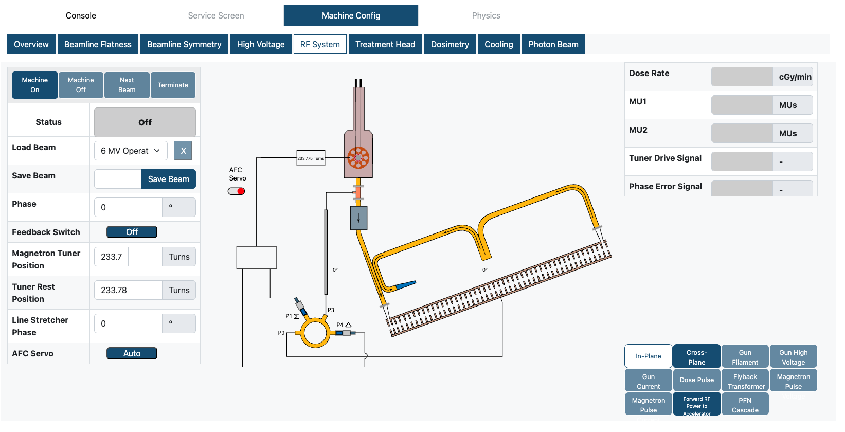
Every screen under Machine Config shares the same frame. Only the inputs column and the schematic change from tab to tab — the controls, status, beam loader, live outputs and plot picker are always in the same place. Learn the frame once here; the rest of this manual covers only what changes per tab. The numbered markers below match the regions in the list.
1
2
3
4
5
6
7
8
9
Representative screen — Elekta · RF System tab. The frame is identical on every Machine Config screen.
1
Application tabs
Switch between the top-level workspaces — Console, Service Screen, Machine Config and Physics.
2
Machine Config tabs
One sub-tab per linac subsystem. The selected tab determines which inputs and schematic are shown. The exact list differs between Varian and Elekta — see the Machine Config overview.
3
Machine & beam controls
Power the simulated linac on or off, start the next beam or terminate the current one. The beam must be on for live outputs to update.
4
Status
Shows whether a beam is currently Off, at Idle, or Delivering.
5
Load / Save Beam
Load a default operating point, or save the current set of inputs as a named beam state for reuse.
6
Inputs column
The editable parameters for the selected subsystem. Each row pairs a value field with its unit; type a value or step it. These are documented per tab in this manual.
7
Subsystem schematic
A live diagram of the selected subsystem. Annotations and meters update as you change inputs while the beam is on.
8
Live outputs
Read-only readouts — always Dose Rate, MU1 and MU2, plus subsystem-specific values such as beam energy, flatness, symmetry or servo signals.
9
Output plots
Selects what the plot displays to reflect the current state of the machine — an internal signal or a water-tank scan of the beam. Click any plot to maximize it; the available plots differ between Varian and Elekta.
The live outputs panel · region 8
Three readouts appear on every tab; the rest depend on the subsystem you are viewing and are listed on each tab's page.
Dose Rate
cGy/min
Physical dose rate delivered at the measurement point.
MU1
MUs
Monitor units accumulated on dosimetry channel 1.
MU2
MUs
Monitor units accumulated on the independent channel 2.
Output plots · region 9
The button grid at the bottom-right selects what the plot displays to reflect the current state of the machine — either an internal signal (gun, magnetron/klystron, PFN…) or a water-tank scan of the beam profile. Click a plot to maximize it. The available plots differ between Varian and Elekta — see Output plots.
Getting started
Anatomy of a Machine Config screen
LAYOUT GUIDE
Every screen under Machine Config shares the same frame. Only the inputs column and the schematic change from tab to tab — the controls, status, beam loader, live outputs and plot picker are always in the same place. Learn the frame once here; the rest of this manual covers only what changes per tab. The numbered markers below match the regions in the list.
1
2
3
4
5
6
7
8
9
Representative screen — Elekta · RF System tab. The frame is identical on every Machine Config screen.
1
Application tabs
Switch between the top-level workspaces — Console, Service Screen, Machine Config and Physics.
2
Machine Config tabs
One sub-tab per linac subsystem. The selected tab determines which inputs and schematic are shown. The exact list differs between Varian and Elekta — see the Machine Config overview.
3
Machine & beam controls
Power the simulated linac on or off, start the next beam or terminate the current one. The beam must be on for live outputs to update.
4
Status
Shows whether a beam is currently Off, at Idle, or Delivering.
5
Load / Save Beam
Load a default operating point, or save the current set of inputs as a named beam state for reuse.
6
Inputs column
The editable parameters for the selected subsystem. Each row pairs a value field with its unit; type a value or step it. These are documented per tab in this manual.
7
Subsystem schematic
A live diagram of the selected subsystem. Annotations and meters update as you change inputs while the beam is on.
8
Live outputs
Read-only readouts — always Dose Rate, MU1 and MU2, plus subsystem-specific values such as beam energy, flatness, symmetry or servo signals.
9
Output plots
Selects what the plot displays to reflect the current state of the machine — an internal signal or a water-tank scan of the beam. Click any plot to maximize it; the available plots differ between Varian and Elekta.
The live outputs panel · region 8
Three readouts appear on every tab; the rest depend on the subsystem you are viewing and are listed on each tab's page.
Dose Rate
cGy/min
Physical dose rate delivered at the measurement point.
MU1
MUs
Monitor units accumulated on dosimetry channel 1.
MU2
MUs
Monitor units accumulated on the independent channel 2.
Output plots · region 9
The button grid at the bottom-right selects what the plot displays to reflect the current state of the machine — either an internal signal (gun, magnetron/klystron, PFN…) or a water-tank scan of the beam profile. Click a plot to maximize it. The available plots differ between Varian and Elekta — see Output plots.
Getting started
Output plots
PLOT REFERENCE VARIAN
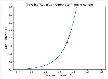
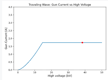
Plots are shared across both simulators unless marked. Characteristic curves (Gun Filament, Gun High Voltage, Gun Grid) plot one quantity against another with a marker at the current operating point; signal plots show a quantity over time.
Showing the plots available on Varian. Click any plot to maximize it.
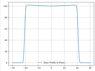
In-Plane
Water-tank scan
x Off-axis position (cm)
y Relative dose (%)
Water-tank dose profile along the in-plane (gun–target) axis. Read flatness and symmetry off the shoulders; penumbra off the edges.
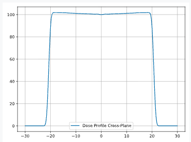
Cross-Plane
Water-tank scan
x Off-axis position (cm)
y Relative dose (%)
Water-tank dose profile along the cross-plane axis, perpendicular to In-Plane.
Gun Filament
Characteristic curve
x Filament current (V)
y Gun current (A)
Gun emission against filament drive. The red marker is the current operating point on the curve.
Gun High Voltage
Characteristic curve
x High voltage (kV)
y Gun current (A)
Gun emission against gun high voltage, showing the space-charge-limited knee. Marker = operating point.
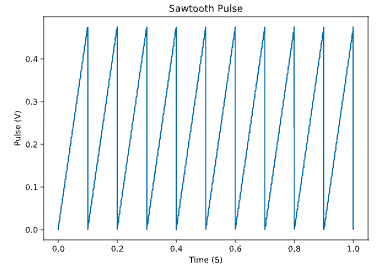
Dose Pulse
Signal vs time
x Time (s)
y Pulse (V)
Ion-chamber dose pulses over time. Each tooth is one beam pulse charging then bleeding off the integrator.
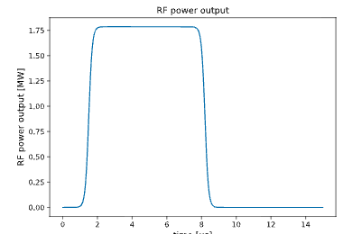
Forward RF Power
Signal vs time
x Time (µs)
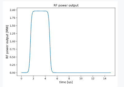
y RF power output (MW)
Forward RF power delivered to the accelerating waveguide during the pulse.
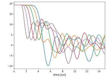
PFN Cascade
Signal vs time
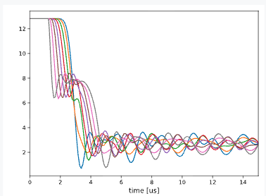
x Time (µs)
y Node voltage (kV)
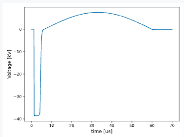
Voltage at each LC node of the pulse-forming network as it discharges — the cascade that shapes the flat HV pulse.
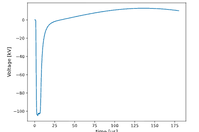
Klystron Pulse Voltage
Signal vs time
x Time (µs)
y Voltage (kV)
Pulse voltage delivered to the klystron (Varian uses a klystron RF amplifier in place of a magnetron).
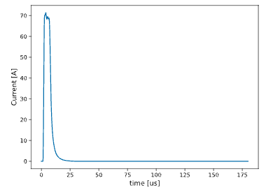
Klystron Pulse Current
Signal vs time
x Time (µs)
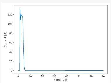
y Current (A)
Pulse current drawn by the klystron during the RF pulse.
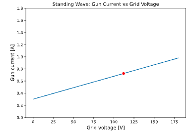
Gun Grid
Characteristic curve
x Grid voltage (V)
y Gun current (A)
Gun emission against grid voltage — the triode gun's control characteristic. Elekta's diode gun has no grid, so this plot is Varian-only.
RF Reflected Pulse
Signal vs time
x Time (µs)
y Current (A)
Reflected RF / gun-current pulse over time, used to judge how well the load is matched.
Not available on Varian
These plots exist only on the other simulator — they reflect hardware Varian does not have (for example, a klystron vs a magnetron, or a triode vs a diode gun).
Gun Current Pulse · Elekta only
Flyback Transformer · Elekta only
Magnetron Pulse Voltage · Elekta only
Magnetron Pulse Current · Elekta only
Getting started
Output plots
PLOT REFERENCE ELEKTA
Plots are shared across both simulators unless marked. Characteristic curves (Gun Filament, Gun High Voltage, Gun Grid) plot one quantity against another with a marker at the current operating point; signal plots show a quantity over time.
Showing the plots available on Elekta. Click any plot to maximize it on the platform. Export any data to CSV.
In-Plane
Water-tank scan
x Off-axis position (cm)
y Relative dose (%)
Water-tank dose profile along the in-plane (gun–target) axis. Read flatness and symmetry off the shoulders; penumbra off the edges.
Cross-Plane
Water-tank scan
x Off-axis position (cm)
y Relative dose (%)
Water-tank dose profile along the cross-plane axis, perpendicular to In-Plane.
Gun Filament
Characteristic curve
x Filament current (V)
y Gun current (A)
Gun emission against filament drive. The red marker is the current operating point on the curve.
Gun High Voltage
Characteristic curve
x High voltage (kV)
y Gun current (A)
Gun emission against gun high voltage, showing the space-charge-limited knee. Marker = operating point.
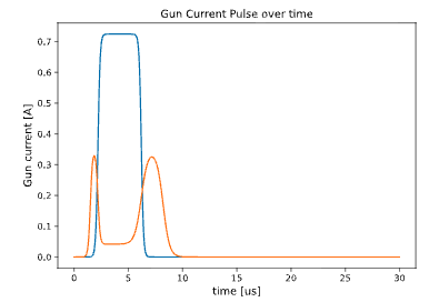
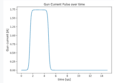
Gun Current Pulse
Signal vs time
x Time (µs)
y Gun current (A)
Shape of a single gun-current pulse over time — rise, flat-top and fall.
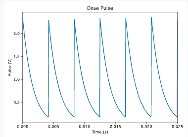
Dose Pulse
Signal vs time
x Time (s)
y Pulse (V)
Ion-chamber dose pulses over time. Each tooth is one beam pulse charging then bleeding off the integrator.
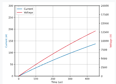
Flyback Transformer
Signal vs time
x Time (µs)
y Current (A) / Voltage (V)
Charging current (left axis) and voltage (right axis) of the flyback transformer during a charge cycle.
Magnetron Pulse Voltage
Signal vs time
x Time (µs)
y Voltage (kV)
Pulse voltage delivered to the magnetron — the discharge of the PFN through the pulse transformer.
Magnetron Pulse Current
Signal vs time
x Time (µs)
y Current (A)
Pulse current drawn by the magnetron during the RF pulse.
Forward RF Power
Signal vs time
x Time (µs)
y RF power output (MW)
Forward RF power delivered to the accelerating waveguide during the pulse.
PFN Cascade
Signal vs time
x Time (µs)
y Node voltage (kV)
Voltage at each LC node of the pulse-forming network as it discharges — the cascade that shapes the flat HV pulse.
Not available on Elekta
These plots exist only on the other simulator — they reflect hardware Elekta does not have (for example, a klystron vs a magnetron, or a triode vs a diode gun).
Klystron Pulse Voltage · Varian only
Klystron Pulse Current · Varian only
Gun Grid · Varian only
RF Reflected Pulse · Varian only
How-to guide
Running and Saving Beams
Load a beam, choose energy, read the first outputs
GUIDE 01
Goal
Get the simulator producing a known beam so you have a stable starting point before changing anything.
1
Power on
On any Machine Config tab, press Machine On in the controls block. Status changes from Off toward ready.
2
Load an operating point
Use Load Beam and pick a saved beam (e.g. "6 MV Operating"). This sets every input across all tabs at once for that energy — gun, RF, steering, bending magnet and treatment head.
Overview →
3
Start the beam
Press Next Beam (Varian) or Beam On (Elekta). The schematic animates and the live-outputs panel begins updating.
4
Read the headline outputs
Check Dose Rate, MU1 and MU2 on the right. These should settle to the values expected for the loaded energy.
Dosimetry →
5
Edit parameters to change your outputs
Edit any parameters to investigate the change to your plots.
6
Save your beam
Type a name beside Save Beam and save, so you can return to this exact state after experimenting or send to other platform sections.
Tips
Loading a beam is the fastest way to a valid machine state — start there rather than typing inputs by hand.
Field size is not changed by loading a beam; set jaws on the Treatment Head tab or the console.
Related tabs
Overview
Dosimetry
Treatment Head
How-to guide
Running and Saving Beams
Load a beam, choose energy, read the first outputs
GUIDE 01
Goal
Get the simulator producing a known beam so you have a stable starting point before changing anything.
1
Power on
On any Machine Config tab, press Machine On in the controls block. Status changes from Off toward ready.
2
Load an operating point
Use Load Beam and pick a saved beam (e.g. "6 MV Operating"). This sets every input across all tabs at once for that energy — gun, RF, steering, bending magnet and treatment head.
Overview →
3
Start the beam
Press Next Beam (Varian) or Beam On (Elekta). The schematic animates and the live-outputs panel begins updating.
4
Read the headline outputs
Check Dose Rate, MU1 and MU2 on the right. These should settle to the values expected for the loaded energy.
Dosimetry →
5
Edit parameters to change your outputs
Edit any parameters to investigate the change to your plots.
6
Save your beam
Type a name beside Save Beam and save, so you can return to this exact state after experimenting or send to other platform sections.
Tips
Loading a beam is the fastest way to a valid machine state — start there rather than typing inputs by hand.
Field size is not changed by loading a beam; set jaws on the Treatment Head tab or the console.
Related tabs
Overview
Dosimetry
Treatment Head
Getting started
Servos
SERVOS
Several subsystems carry a servo — a closed feedback loop that watches an output and continuously trims its input to hold the beam at its operating point. Every servo can be switched on or off, and that switch decides whether the simulator corrects your changes or lets them stand.
Servos on
The corresponding outputs servo back toward their default. Change an input and the loop works against you, pulling the beam back to where it started — the same way a real machine holds its output steady through a treatment.
Servos off
Nothing corrects for you. A change travels straight through to the outputs and stays there, so you can investigate cause and effect without the loop hiding it. This is the setting to use when learning how one input moves an output.
Losing the beam is not always reversible
With the servos off it is possible to drive the machine into a state where dose is being lost. If enough pulses are delivered in that state, returning the input to a proper operating point may not bring the beam back — the machine cannot always recover on its own. When that happens, load a saved beam to return to a known-good state.
Where you will find them
Steering servos
On Beamline Symmetry — drive the steering coils to hold radial and transverse symmetry. Turn them off before hand-steering the beam.
AFC servo
On RF System — holds the drive frequency on the accelerator's resonance. With it off, the tuner stays where you put it and the phase error is yours to read.
Gun and dose servos
On Dosimetry — hold dose rate steady by trimming the gun current against the monitor-chamber reading.
PFN servo
On the high-voltage screens — calculates the PFN voltage for the requested operating point rather than taking it directly from you.
See also
Beamline Symmetry
RF System
Dosimetry
Tune flatness & symmetry
Getting started
Servos
SERVOS
Several subsystems carry a servo — a closed feedback loop that watches an output and continuously trims its input to hold the beam at its operating point. Every servo can be switched on or off, and that switch decides whether the simulator corrects your changes or lets them stand.
Servos on
The corresponding outputs servo back toward their default. Change an input and the loop works against you, pulling the beam back to where it started — the same way a real machine holds its output steady through a treatment.
Servos off
Nothing corrects for you. A change travels straight through to the outputs and stays there, so you can investigate cause and effect without the loop hiding it. This is the setting to use when learning how one input moves an output.
Losing the beam is not always reversible
With the servos off it is possible to drive the machine into a state where dose is being lost. If enough pulses are delivered in that state, returning the input to a proper operating point may not bring the beam back — the machine cannot always recover on its own. When that happens, load a saved beam to return to a known-good state.
Where you will find them
Steering servos
On Beamline Symmetry — drive the steering coils to hold radial and transverse symmetry. Turn them off before hand-steering the beam.
AFC servo
On RF System — holds the drive frequency on the accelerator's resonance. With it off, the tuner stays where you put it and the phase error is yours to read.
Gun and dose servos
On Dosimetry — hold dose rate steady by trimming the gun current against the monitor-chamber reading.
PFN servo
On the high-voltage screens — calculates the PFN voltage for the requested operating point rather than taking it directly from you.
See also
Beamline Symmetry
RF System
Dosimetry
Tune flatness & symmetry
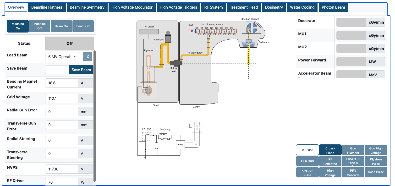
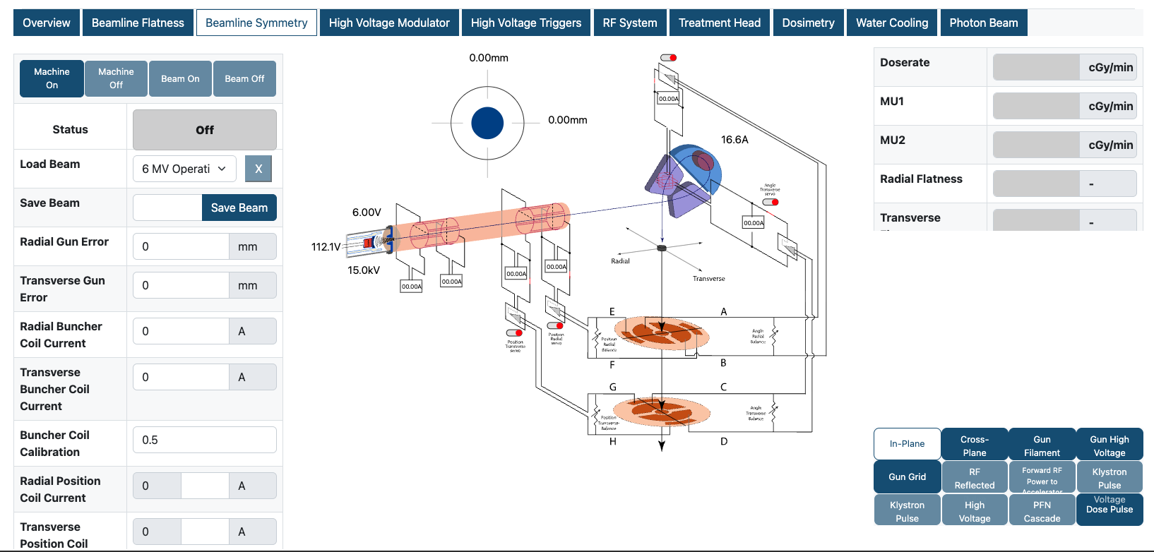
Varian · Machine Config
Overview
TAB 01 VARIAN
A consolidated cockpit: the most-used inputs from across the beamline on one screen, with the full gun-to-target schematic. Load a beam and confirm output here before drilling into a subsystem.
Default values may be slightly off as changes are released to the simulator and its beam models. Treat them as a starting point rather than a fixed reference.
Inputs
Parameter
Default 6 MV10 MV15 MV
Range
What it does
Bending Magnet Current
16.626.639A
11.5 – 100
Current through the bending magnet; selects electron energy.
Grid Voltage
112.1112.191.7V
-80 – 180
Triode-gun grid voltage; regulates the rate electrons leave the gun.
Radial Steering
000A
-300 – 300
Combined radial steering current applied from the Overview screen.
Transverse Steering
000A
-300 – 300
Combined transverse steering current applied from the Overview screen.
HVPS
117301173013200V
10000 – 16000
High voltage supplied to the PFN circuit.
RF Driver
707070W
40 – 200
Power supplied to the klystron.
Outputs
Dose Rate, MU1 and MU2 appear on every tab; the rest are specific to this subsystem.
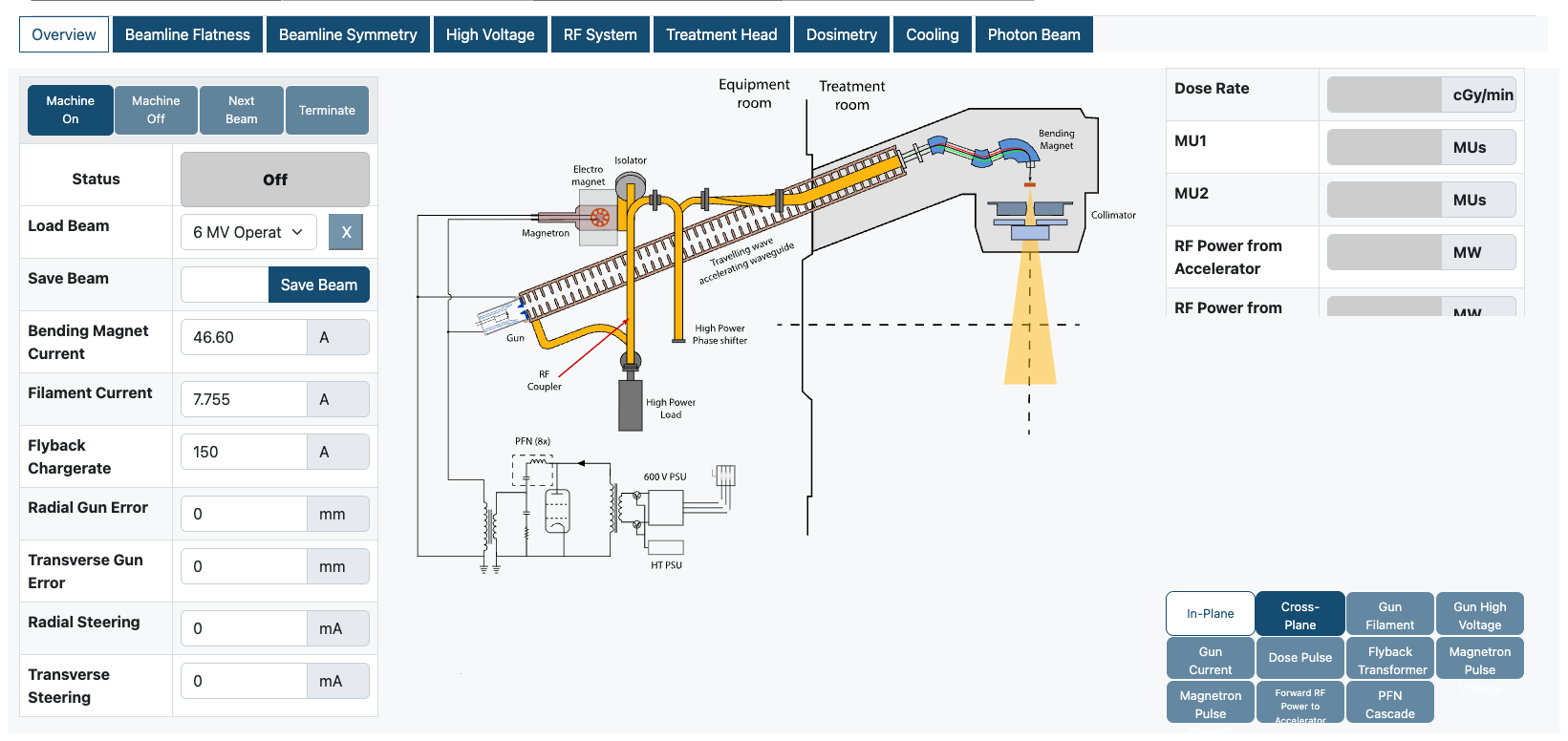
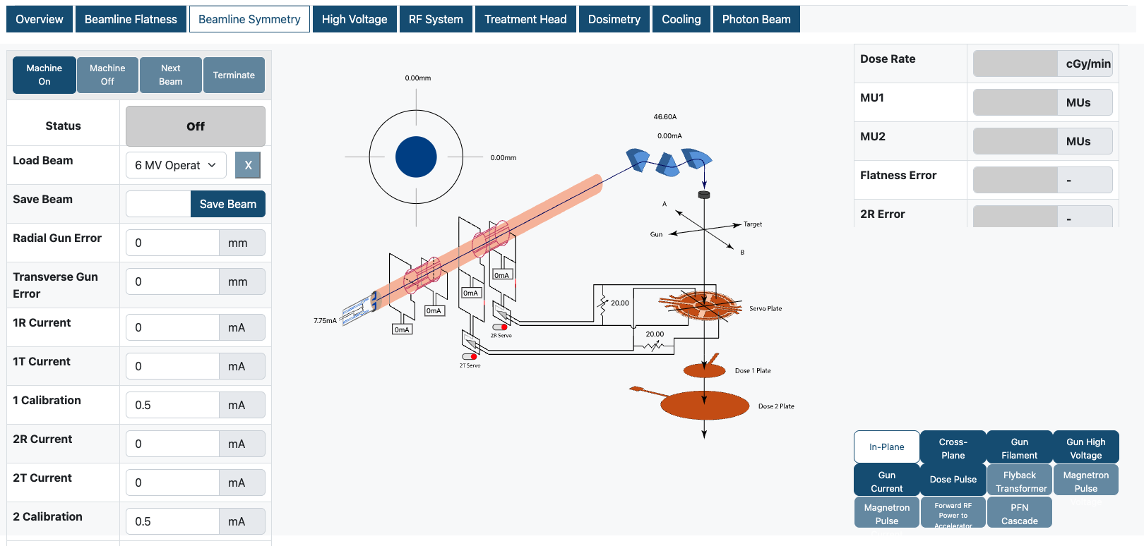
A consolidated cockpit gathering the most-used inputs across the beamline, with the full gun-to-target schematic. Load a beam and confirm output here before drilling into a subsystem.
Default values may be slightly off as changes are released to the simulator and its beam models. Treat them as a starting point rather than a fixed reference.
Inputs
Parameter
Default 6 MV10 MV15 MV
Range
What it does
Bending Magnet Current
46.672.8105.5A
33.5 – 140
Current through the bending magnet; selects electron energy.
Filament Current
7.7557.57.67A
7 – 8
Current supplied to the electron-gun filament.
Flyback Chargerate
150150204A
0 – 1000
Current used in the flyback charging cycle.
Radial Steering
000mA
-300 – 300
Combined radial steering current applied from the Overview screen.
Transverse Steering
000mA
-300 – 300
Combined transverse steering current applied from the Overview screen.
Outputs
Dose Rate, MU1 and MU2 appear on every tab; the rest are specific to this subsystem.
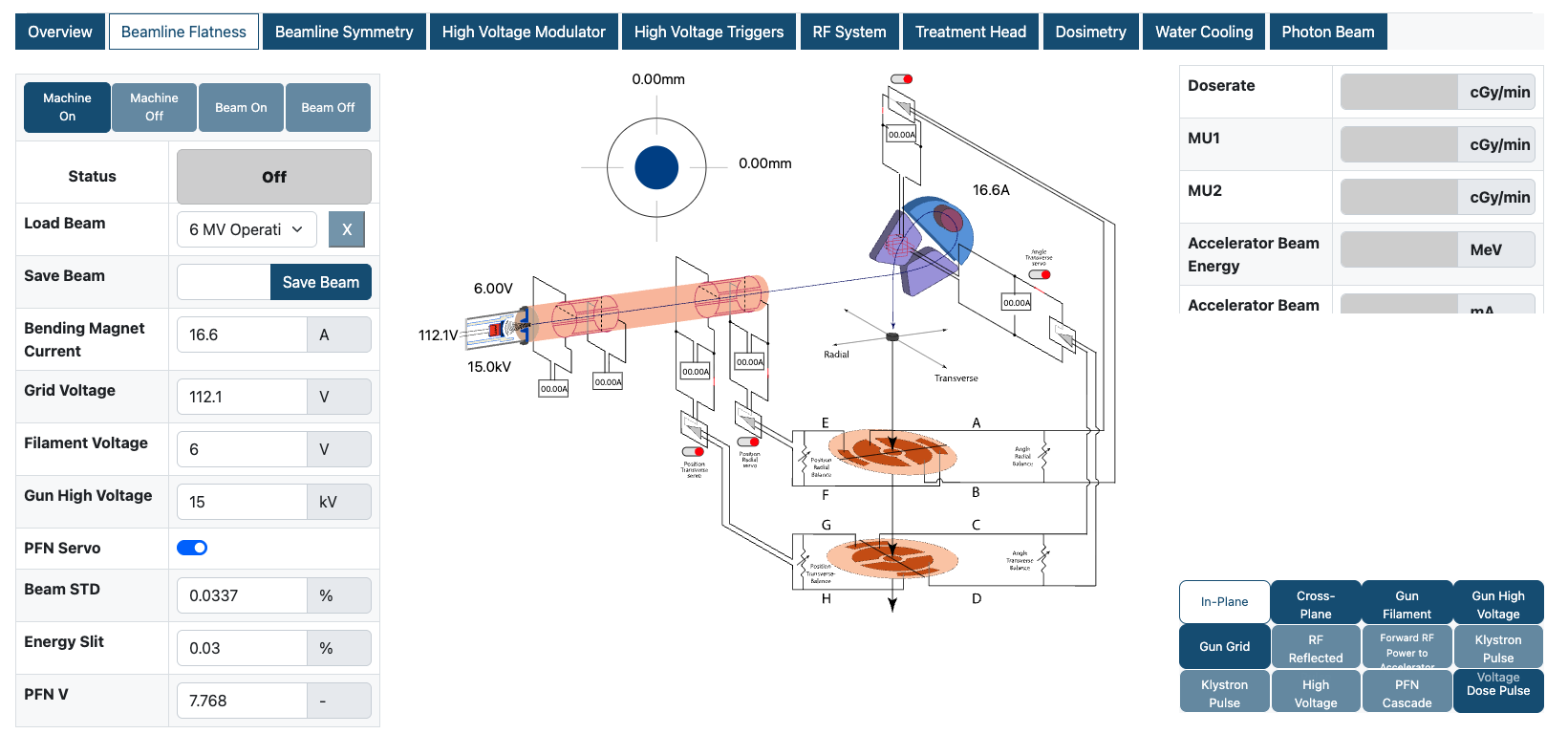
Controls the electron source and energy selection — the inputs that shape penetration and the off-axis profile. Steering for symmetry lives on the next tab.
Inputs
Parameter
Default 6 MV10 MV15 MV
Range
What it does
Bending Magnet Current
16.626.639A
11.5 – 100
Current through the bending magnet; selects electron energy.
Grid Voltage
112.1112.191.7V
-80 – 180
Triode-gun grid voltage; regulates the rate electrons leave the gun.
Filament Voltage
666V
4.8 – 6.3
Higher filament voltage raises filament temperature, increasing electron emission.
Gun High Voltage
151510kV
0 – 20
Gun emission against gun high voltage, showing the space-charge-limited knee. Marker = operating point.
PFN V
7.7688.658.72kV
0 - 10
Desired voltage on the PFN.
Outputs
Dose Rate, MU1 and MU2 appear on every tab; the rest are specific to this subsystem.
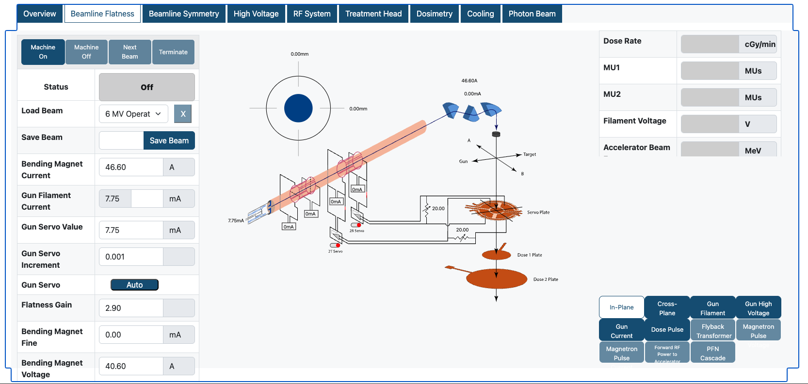
Controls the electron source and energy selection — the inputs that shape penetration and the off-axis profile, plus the gun servo and focus coils. Steering for symmetry lives on the next tab.
Inputs
Parameter
Default 6 MV10 MV15 MV
Range
What it does
Bending Magnet Current
46.672.8105.5A
33.5 – 140
Current through the bending magnet; selects electron energy.
Gun Filament Current
7.757.57.67mA
0 – 1000
Current supplied to the gun filament; sets emission.
Gun Servo Value
7.757.57.67mA
0 – 1000
Weighted gun-current value the servo holds at equilibrium.
Gun Servo Increment
0.0010.0010.001
0 – 10
Step size of the gun servo loop.
Flatness Gain
2.93.463.95
-300 – 300
Scale factor comparing inner vs outer monitor-chamber segments (hump balance).
Bending Magnet Fine
000mA
-300 – 300
Fine-control current on the bending-magnet coil.
Bending Magnet Voltage
40.640.640.6A
-300 – 300
Voltage across the bending-magnet coil.
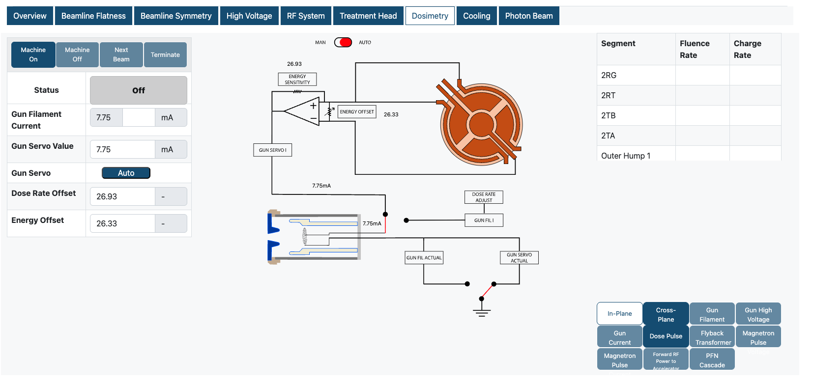
Dose Rate Offset
26.9326.9326.93
0 – 4000
Offset applied to measured dose in the monitor chamber.
Energy Offset
26.3326.3326.33
0 – 4000
Energy offset applied via the monitor chamber.
Outputs
Dose Rate, MU1 and MU2 appear on every tab; the rest are specific to this subsystem.
All beam steering — the three coil pairs down the waveguide plus their calibrations and servos. The buncher coils (gun end) are the most sensitive; angle coils sit nearest the target.
Inputs
Parameter
Default 6 MV10 MV15 MV
Range
What it does
Radial Buncher Coil Current
000A
-300 – 300
Most sensitive steering coils, at the gun end of the waveguide (radial).
Transverse Buncher Coil Current
000A
-300 – 300
Buncher steering at the gun end (transverse).
Radial Position Coil Current
000A
-300 – 300
Position steering at the waveguide exit (radial); sets beam position on the target.
Transverse Position Coil Current
000A
-300 – 300
Position steering at the waveguide exit (transverse).
Radial Angle Coil Current
000A
-300 – 300
Angle steering near the target (radial); sets the beam incidence angle.
Transverse Angle Coil Current
000A
-300 – 300
Angle steering near the target (transverse).
Outputs
Dose Rate, MU1 and MU2 appear on every tab; the rest are specific to this subsystem.
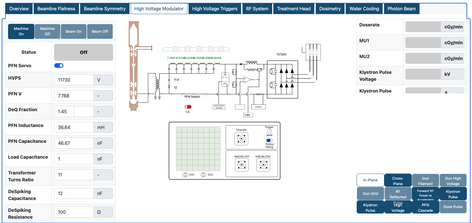
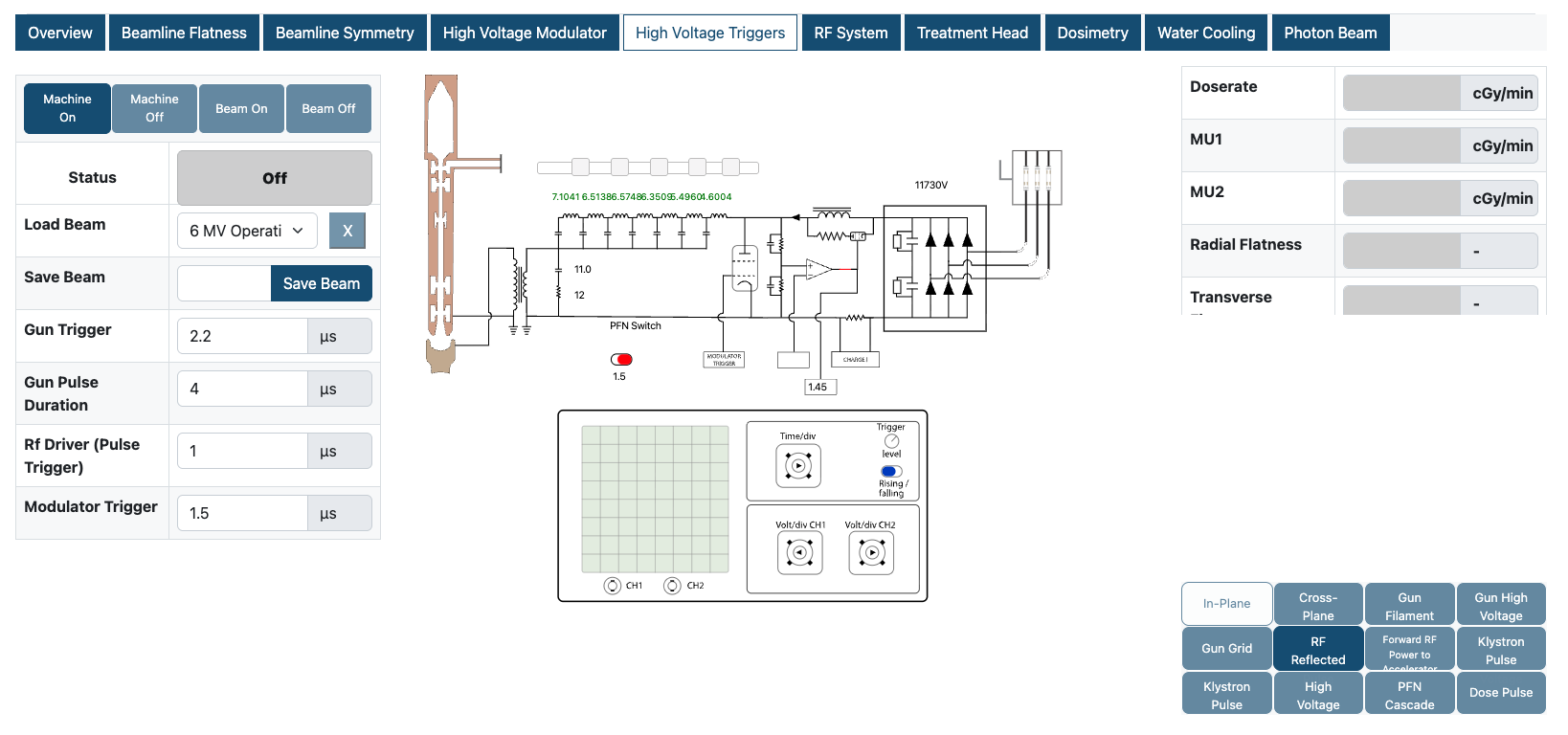
The PFN circuit: charges the pulse-forming network and discharges it through the klystron to form each RF pulse. Set the charging supply and PFN component values here.
Inputs
Parameter
Default 6 MV10 MV15 MV
Range
What it does
HVPS
117301173013200V
10000 – 16000
High voltage supplied to the PFN circuit.
PFN V
7.7688.658.72kV
0 – 20
Desired voltage on the PFN.
DeQ Fraction
1.451.631.45
1 – 2
How much of a de-Q-ing charge cycle completes; sets the PFN voltage.
DeSpiking Capacitance
121212nF
0 – 1000
Capacitance of the de-spiking network capacitor.
DeSpiking Resistance
100100100Ω
0 – 1000
Resistance of the de-spiking network resistor.
Outputs
Dose Rate, MU1 and MU2 appear on every tab; the rest are specific to this subsystem.
Doserate
cGy/min
Physical dose rate at the measurement point.
MU1
MUs
Monitor units on dosimetry channel 1.
MU2
MUs
Monitor units on the independent channel 2.
Klystron Pulse Voltage
kV
Pulse voltage applied to the klystron.
Klystron Pulse Current
A
Pulse current applied to the klystron.
DeQ Pulse Voltage
kV
Voltage delivered by the de-Q-ing circuit into the PFN.
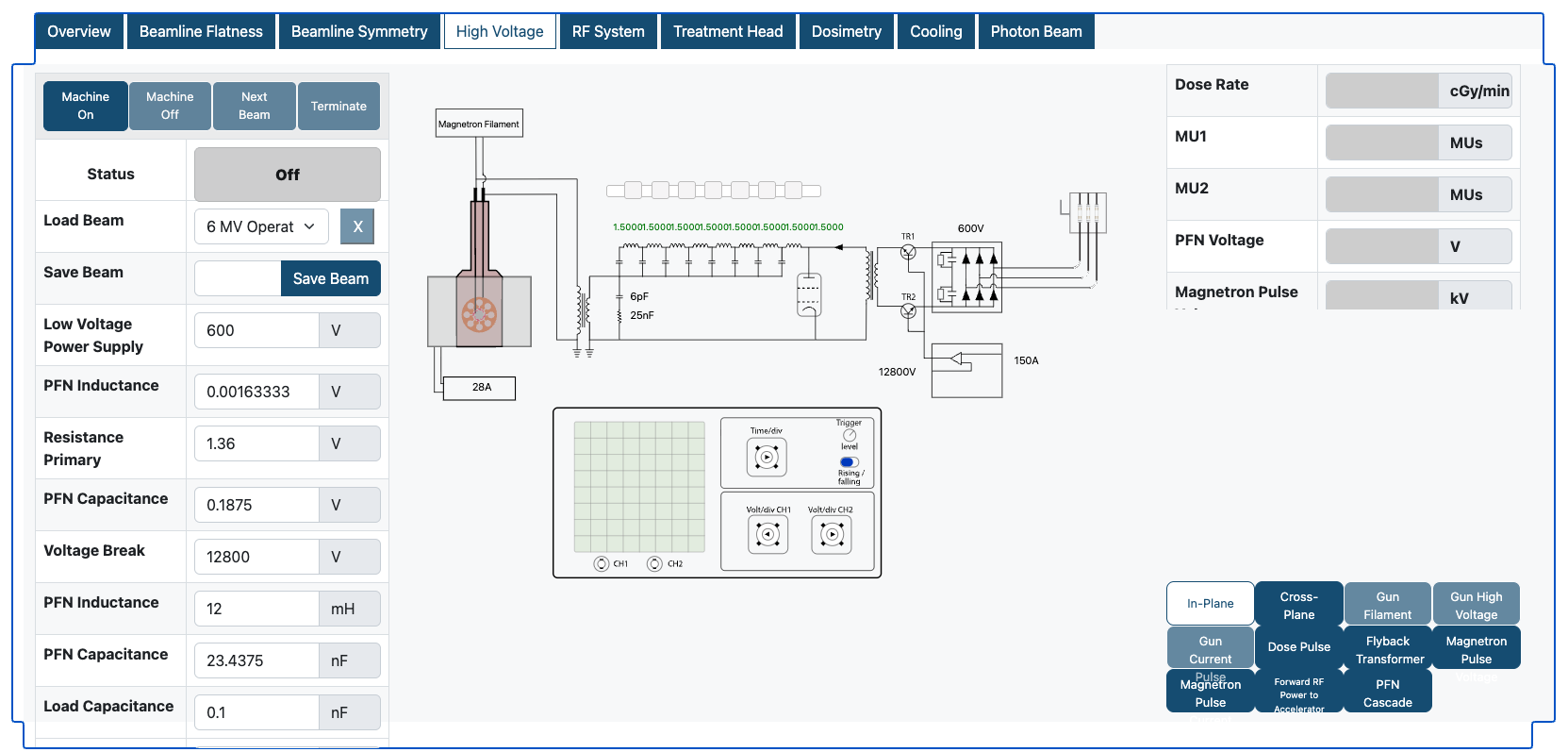
The modulator charges the pulse-forming network (PFN) and discharges it through the magnetron to form each RF pulse. Set the charging supply and PFN component values here.
Inputs
Parameter
Default 6 MV10 MV15 MV
Range
What it does
Low Voltage Power Supply
600600600V
0 – 17000
Low-voltage supply feeding the flyback transformer.
Resistance Primary
1.361.361.36Ω
0 – 1000
Resistance of the pulse-transformer primary winding circuit.
Voltage Break
128001302020000V
0 – 20000
Upper voltage set-point of the flyback transformer for the PFN.
PFN Inductance
121212mH
0 – 1000
Total inductance of the series inductors in the PFN discharge cycle.
PFN Capacitance
23.437523.437523.4375nF
0 – 1000
Total capacitance of the parallel capacitors in the PFN discharge cycle.
Electromagnet
283033A
28 – 35
Current supplied to the magnetron electromagnet.
DeSpiking Capacitance
666nF
0 – 1000
Capacitance of the de-spiking network capacitor.
DeSpiking Resistance
252525Ω
0 – 1000
Resistance of the de-spiking network resistor.
Flyback Chargerate
150150204A
0 – 1000
Current used in the flyback charging cycle.
Outputs
Dose Rate, MU1 and MU2 appear on every tab; the rest are specific to this subsystem.
Pulse timing for the modulator: the start times and durations that sequence the RF driver, the PFN discharge and the gun pulse against the main trigger.
Inputs
Parameter
Default 6 MV10 MV15 MV
Range
What it does
Gun Trigger
2.22.22.2µs
0 – 20
Start time of the gun pulse relative to the main trigger.
Gun Pulse Duration
444µs
0 – 20
Duration of the gun pulse.
RF Driver Pulse Trigger
111µs
0 – 20
Start time of the RF-driver pulse relative to the main trigger.
Modulator Trigger
1.51.51.5µs
0 – 20
Start time of the PFN discharge relative to the main trigger.
Outputs
Dose Rate, MU1 and MU2 appear on every tab; the rest are specific to this subsystem.
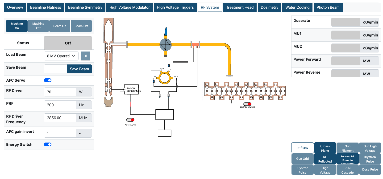
Generates and tunes the RF that accelerates the beam. The AFC (Automatic Frequency Control) servo keeps the drive frequency on the accelerator's resonance as the machine warms.
Inputs
Parameter
Default 6 MV10 MV15 MV
Range
What it does
RF Driver
707070W
40 – 200
Power supplied to the klystron.
PRF
200200200Hz
0 – 1000
Pulse repetition frequency — RF pulses per second.
RF Driver Frequency
285628562856MHz
0 – 4000
Drive frequency when the machine is cold.
Outputs
Dose Rate, MU1 and MU2 appear on every tab; the rest are specific to this subsystem.
Tunes the magnetron and the AFC servo that keeps it on the accelerator's resonance. The tuner position and line-stretcher phase set the operating point; the AFC servo can hold it automatically.
Inputs
Parameter
Default 6 MV10 MV15 MV
Range
What it does
Phase
000°
-180 – 180
Phase shift of RF in the high-power feedback loop between accelerator exit and entrance.
Magnetron Tuner Position
233.775233.775233.775Turns
0 – 4000
Number of turns on the magnetron tuner.
Tuner Rest Position
233.78233.78233.78Turns
0 – 4000
Initial turns setting for the magnetron tuner.
Line Stretcher Phase
000°
0 – 4000
Low-power phase offset for hybrid-ring port 3.
Outputs
Dose Rate, MU1 and MU2 appear on every tab; the rest are specific to this subsystem.
Dose Rate
cGy/min
Physical dose rate at the measurement point.
MU1
MUs
Monitor units on dosimetry channel 1.
MU2
MUs
Monitor units on the independent channel 2.
Tuner Drive Signal
—
AFC tuner drive output.
Phase Error Signal
—
Phase error sensed by the AFC servo.
Hybrid Ring Port 4
—
Signal at hybrid-ring port 4 of the phase circulator.
Hybrid Ring Port 1
—
Signal at hybrid-ring port 1 of the phase circulator.
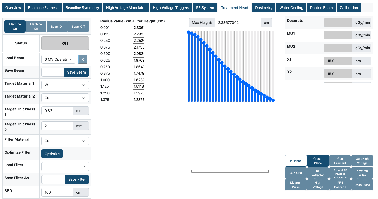
Photon production and beam shaping downstream of the bending magnet: target, flattening filter, monitor chamber and the collimator jaws that set field size.
Inputs
Parameter
Default
Range
What it does
Target Material 1dropdown
W
—
Material of the first target layer.
Target Material 2dropdown
Cu
—
Material of the second target layer.
Target Thickness 1
0.82 mm
0 – 50
Thickness of the first target layer.
Target Thickness 2
2 mm
0 – 50
Thickness of the second target layer (0 for a single material).
Optimize Filterbutton
—
—
Re-optimizes the filter shape for a flat profile after energy/target/filter changes.
FFF Flagcheckbox
Off
—
Operate flattened (FF) or flattening-filter-free (FFF).
Filter Materialdropdown
Cu
—
Flattening-filter material.
X Elevation
36.7 cm
0 – 50
Distance of the X jaws from the source.
Y Elevation
28 cm
0 – 50
Distance of the Y jaws from the source.
SSD
100 cm
80 – 120
Source-to-surface distance.
Scatter Flagcheckbox
On
—
Include scatter calculations.
X1 / X2
20 cm
2 – 20
X-axis jaw positions. Model accuracy drops below 5 × 5 cm.
Y1 / Y2
20 cm
2 – 20
Y-axis jaw positions. Model accuracy drops below 5 × 5 cm.
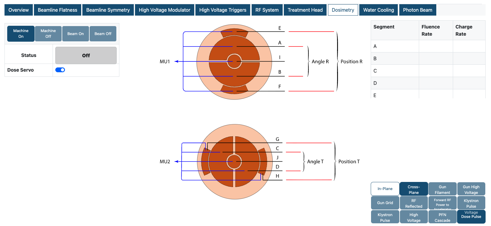
The monitor (ion) chamber and dose servo. The chamber is split into segments (A–J) whose charges combine into the two dose channels and the symmetry/flatness error signals.
Inputs
Parameter
Default
Range
What it does
Dose Servotoggle
On
—
Closed-loop control that holds dose rate steady by adjusting gun current.
Outputs
Dose Rate, MU1 and MU2 appear on every tab; the rest are specific to this subsystem.
A
charge
Charge collected on monitor-chamber segment A.
B
charge
Charge collected on monitor-chamber segment B.
C
charge
Charge collected on monitor-chamber segment C.
D
charge
Charge collected on monitor-chamber segment D.
E
charge
Charge collected on monitor-chamber segment E.
F
charge
Charge collected on monitor-chamber segment F.
G
charge
Charge collected on monitor-chamber segment G.
H
charge
Charge collected on monitor-chamber segment H.
I
charge
Charge collected on monitor-chamber segment I.
J
charge
Charge collected on monitor-chamber segment J.
Dose 1 = A + B + E + F + I
MU
Dose channel 1 — sum of segments A, B, E, F, I.
Dose 2 = C + D + G + H + J
MU
Dose channel 2 — sum of segments C, D, G, H, J.
Sym Angle Radial
—
Radial angle-symmetry error from the segments.
Sym Angle Trans
—
Transverse angle-symmetry error.
Sym Position Radial
—
Radial position-symmetry error.
Sym Position Trans
—
Transverse position-symmetry error.
Flat rad
—
Radial flatness error derived from inner vs outer segments.
The monitor (ion) chamber and gun servo. The chamber's hump and dose segments measure uniformity; their offsets feed the gun servo that holds output steady.
Inputs
Parameter
Default 6 MV10 MV15 MV
Range
What it does
Gun Filament Current
7.757.57.67mA
0 – 1000
Current supplied to the gun filament; sets emission.
Gun Servo Value
7.757.57.67mA
0 – 1000
Weighted gun-current value the servo holds at equilibrium.
Dose Rate Offset
26.9326.9326.93
0 – 4000
Offset applied to measured dose in the monitor chamber.
Energy Offset
26.3326.3326.33
0 – 4000
Energy offset applied via the monitor chamber.
Outputs
Dose Rate, MU1 and MU2 appear on every tab; the rest are specific to this subsystem.
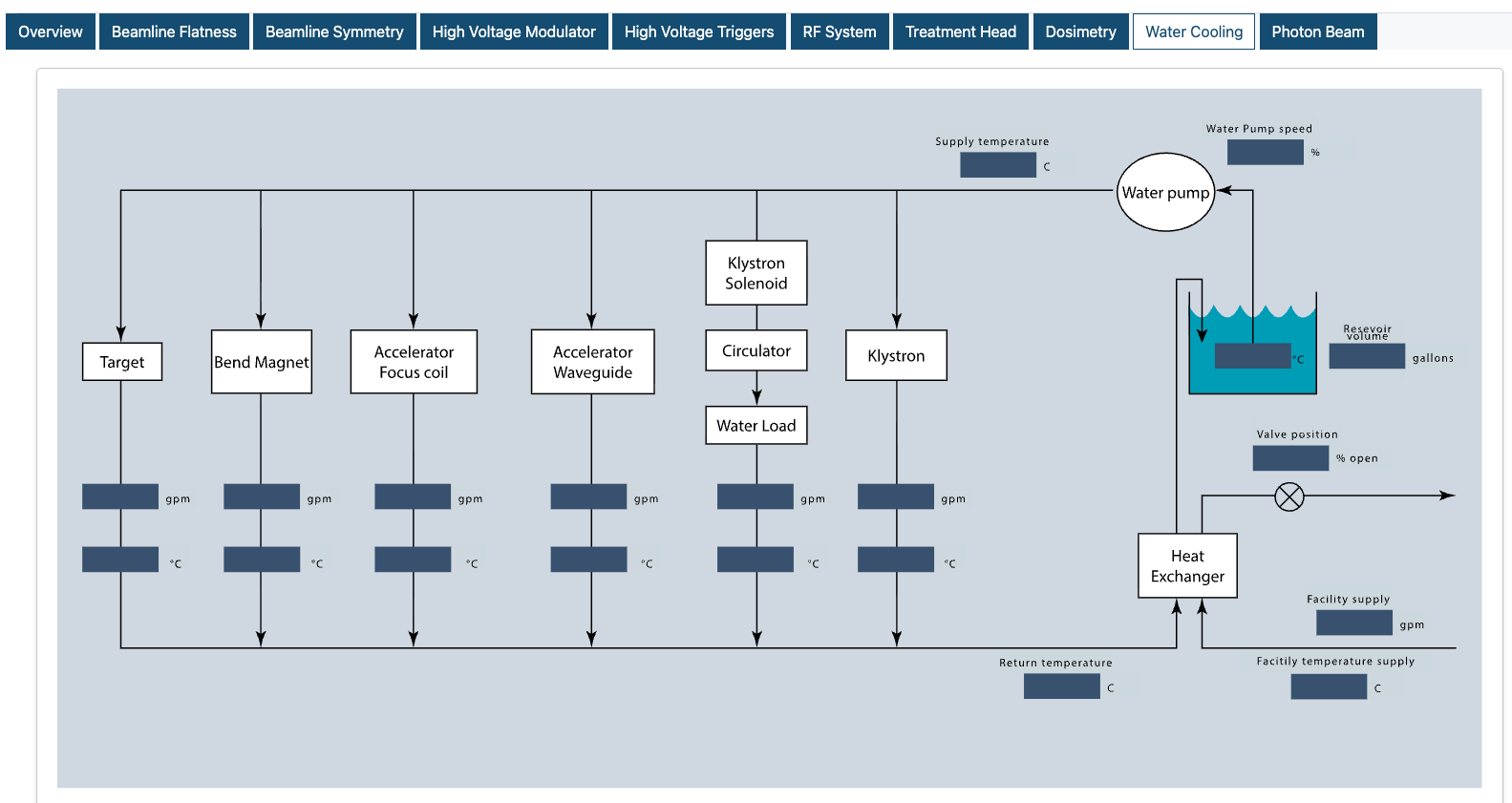
A block diagram of the cooling loop that removes heat from each linac subsystem through a heat exchanger and reservoir. This screen is read-only: every cooled component reports its temperature and coolant flow.
Outputs — per cooled component
Every component on the cooling diagram reports two read-only values: its coolant temperature and flow.
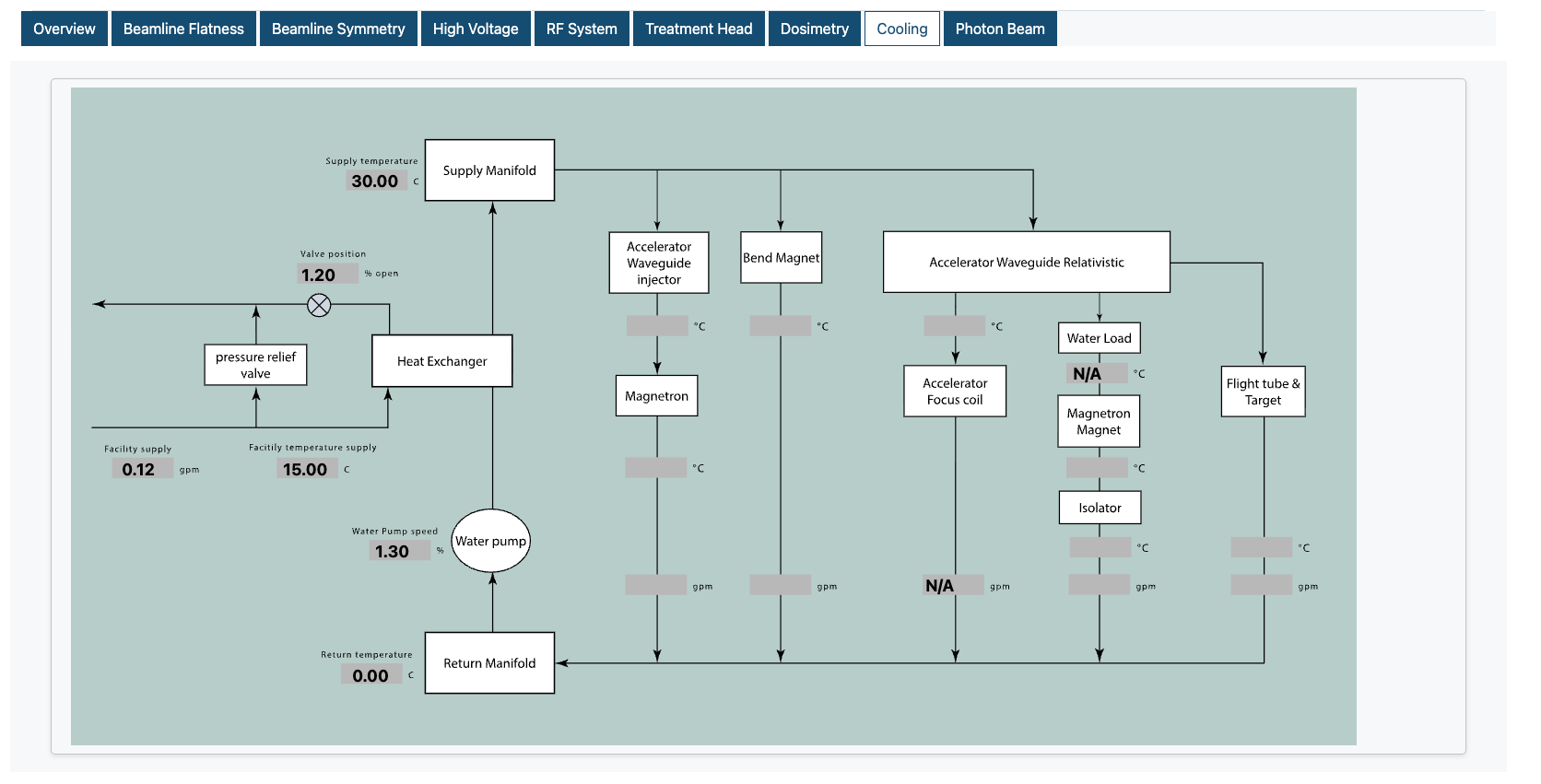
A block diagram of the cooling loop removing heat from each linac subsystem through a heat exchanger and reservoir. This screen is read-only: every cooled component reports its temperature and coolant flow.
Outputs — per cooled component
Every component on the cooling diagram reports two read-only values: its coolant temperature and flow.
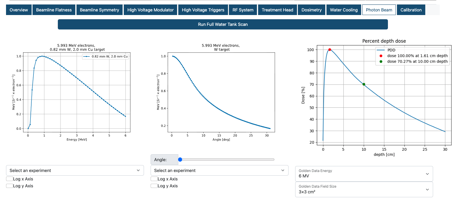
Runs a full water tank scan to produce the photon beam's fluence and its percentage depth dose (PDD). The two left-hand plots show the bremsstrahlung fluence coming off the target — against photon energy, and against emission angle — while the right-hand plot gives the PDD with d-max and the dose at 10 cm marked. The PDD can also be obtained from the Scanning Water Tank.
Inputs
Parameter
Default
Range
What it does
Run Full Water Tank Scanbutton
—
—
Runs the complete scan and populates all three plots for the current beam.
Select an experiment (fluence)dropdown
—
—
Overlays a stored experiment on the energy-fluence plot for comparison.
Select an experiment (angle)dropdown
—
—
Overlays a stored experiment on the angular-fluence plot.
Angle
0 deg
0 – 30
Emission angle at which the energy-fluence spectrum is sampled.
Log x Axis / Log y Axischeckbox
Off
—
Switches either fluence plot to a logarithmic axis.
Golden Data Energydropdown
6 MV
—
Energy of the reference (golden) PDD drawn against your scan.
Golden Data Field Sizedropdown
3×3 cm²
—
Field size of the reference PDD dataset.
Outputs
Dose Rate, MU1 and MU2 appear on every tab; the rest are specific to this subsystem.
Energy Fluence
MeV sr⁻¹ electron⁻¹
Bremsstrahlung fluence against photon energy for the current target stack.
Angular Fluence
MeV sr⁻¹ electron⁻¹
Fluence against emission angle from the target.
Percent Depth Dose
%
Relative dose against depth in water, normalised to d-max.
d-max
cm
Depth of maximum dose, marked on the PDD curve.
Dose at 10 cm
%
Relative dose at 10 cm depth — the common beam-quality checkpoint.
Runs a full water tank scan to produce the photon beam's fluence and its percentage depth dose (PDD). The two left-hand plots show the bremsstrahlung fluence coming off the target — against photon energy, and against emission angle — while the right-hand plot gives the PDD with d-max and the dose at 10 cm marked. The PDD can also be obtained from the Scanning Water Tank.
Inputs
Parameter
Default
Range
What it does
Run Full Water Tank Scanbutton
—
—
Runs the complete scan and populates all three plots for the current beam.
Select an experiment (fluence)dropdown
—
—
Overlays a stored experiment on the energy-fluence plot for comparison.
Select an experiment (angle)dropdown
—
—
Overlays a stored experiment on the angular-fluence plot.
Angle
0 deg
0 – 30
Emission angle at which the energy-fluence spectrum is sampled.
Log x Axis / Log y Axischeckbox
Off
—
Switches either fluence plot to a logarithmic axis.
Golden Data Energydropdown
6 MV
—
Energy of the reference (golden) PDD drawn against your scan.
Golden Data Field Sizedropdown
3×3 cm²
—
Field size of the reference PDD dataset.
Outputs
Dose Rate, MU1 and MU2 appear on every tab; the rest are specific to this subsystem.
Energy Fluence
MeV sr⁻¹ electron⁻¹
Bremsstrahlung fluence against photon energy for the current target stack.
Angular Fluence
MeV sr⁻¹ electron⁻¹
Fluence against emission angle from the target.
Percent Depth Dose
%
Relative dose against depth in water, normalised to d-max.
d-max
cm
Depth of maximum dose, marked on the PDD curve.
Dose at 10 cm
%
Relative dose at 10 cm depth — the common beam-quality checkpoint.
Model-calibration constants: the coil calibration factors, energy-spread and gun-alignment terms, PFN component values and jaw elevations that tie the simulation to a real machine. These are set once for an operating point rather than tuned beam to beam, and several are shared with the Service Mode preset screens.
Inputs
Parameter
Default 6 MV10 MV15 MV
Range
What it does
Beam STD
0.03370.03370.0337%
0 – 2
Energy spread (Gaussian standard deviation, as % of total beam energy).
Energy Slit
0.030.030.03%
0 – 2
Width of the energy slit that trims the spectrum passing the bending magnet.
Radial Gun Error
000mm
0 – 2
Gun-axis misalignment relative to the accelerating section (radial).
Transverse Gun Error
000mm
0 – 2
Gun-axis misalignment relative to the accelerating section (transverse).
Buncher Coil Calibration
0.50.350.25
-300 – 300
Calibration factor for the buncher-coil response.
Position Coil Calibration
0.50.350.25
-300 – 300
Calibration factor for the position-coil response.
Angle Coil Calibration
0.50.350.25
-300 – 300
Calibration factor for the angle-coil response.
PFN Inductance
36.6436.6436.64mH
30 – 40
Total inductance of the series inductors in the PFN discharge cycle.
PFN Capacitance
46.6746.6746.67nF
0 – 1000
Total capacitance of the parallel capacitors in the PFN discharge cycle.
Load Capacitance
111nF
0 – 100
Equivalent capacitance of the klystron load.
Transformer Turns Ratio
111111
1 – 20
Turns ratio of the pulse transformer.
AFC gain invert
111
0 – 100
Inverts the sign of the AFC servo gain, reversing the direction the tuner drives.
Model-calibration constants: the coil calibration factors, energy-spread and gun-alignment terms, PFN component values and jaw elevations that tie the simulation to a real machine.
Inputs
Parameter
Default 6 MV10 MV15 MV
Range
What it does
Beam STD
0.03370.03370.0337%
0 – 2
Energy spread (Gaussian standard deviation, as % of total beam energy).
Energy Slit
0.10.030.03%
0 – 2
Width of the energy slit that trims the spectrum passing the bending magnet.
Radial Gun Error
000mm
0 – 2
Gun-axis misalignment relative to the accelerating section (radial).
Transverse Gun Error
000mm
0 – 2
Gun-axis misalignment relative to the accelerating section (transverse).
1 Calibration
0.50.350.25mA
-300 – 300
Calibration factor matching the 1-coil response to a real linac.
2 Calibration
0.50.350.25mA
-300 – 300
Calibration factor for the 2-coil response.
PFN Inductance
0.001630.001630.00163mH
0 – 1000
Total inductance of the series inductors in the PFN discharge cycle.
PFN Capacitance
0.18750.18750.1875nF
0 – 1000
Total capacitance of the parallel capacitors in the PFN discharge cycle.
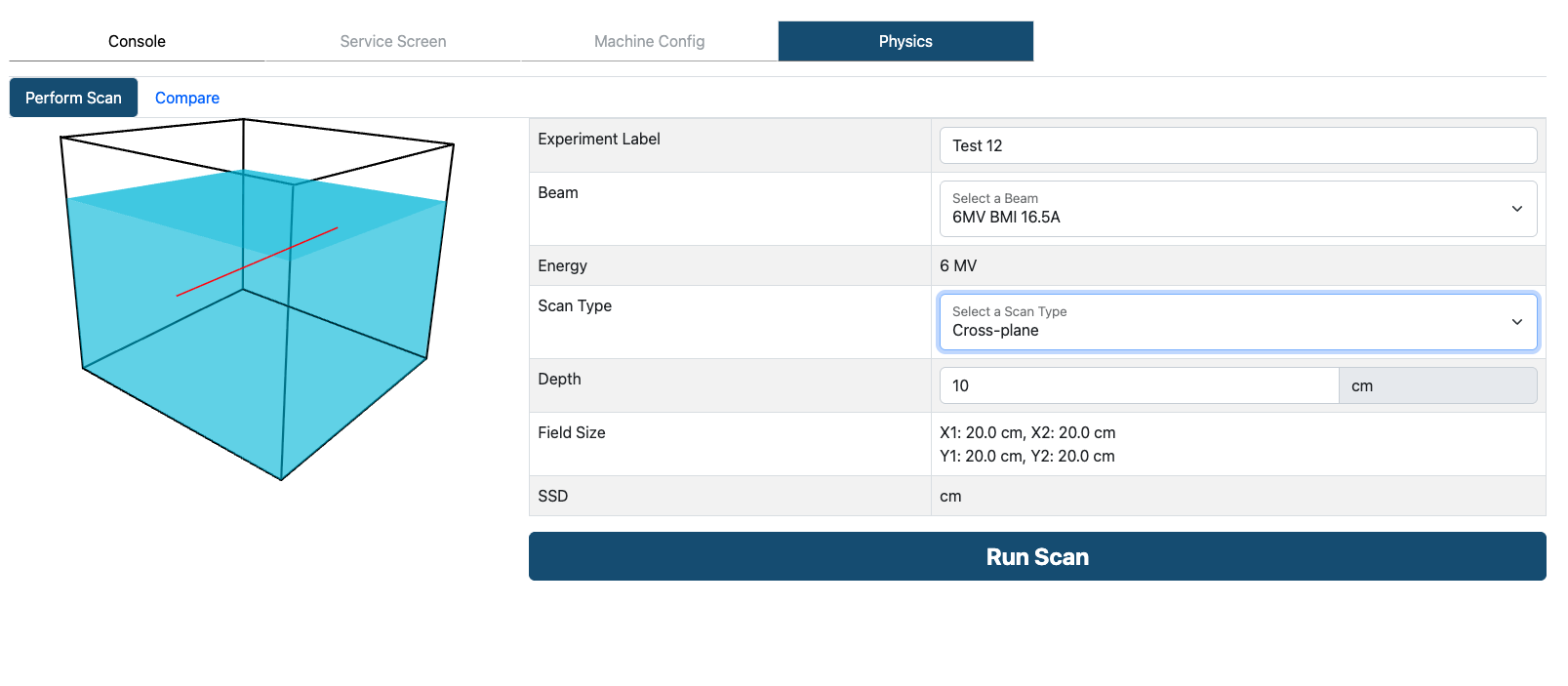
The Scanning Water Tank runs dose scans on any beam you built and saved in Machine Config — no measurement hardware required. Set to Physics Mode → Scanning Water Tank on the Console and then navigate to the Physics tab. Load beams and set up scans in Perform Scan then compare scans on the same plot in Compare.
1
2
3
4
5
6
7
8
9
Numbered markers match the list below.
What each area does
1
Perform Scan / Compare tabs
Switch between running a scan and comparing stored results.
2
Tank view
3-D view of the water tank; the red line shows the scan axis for the selected scan type.
3
Experiment Label
Name the scan so you can find it later on the Compare tab.
4
Beam
Select a default beam or one of the operating points you saved in Machine Config.
5
Energy
Read-only — follows the selected beam (MV).
6
Scan Type
Choose the profile to acquire: In-Plane, Cross-Plane or Depth (PDD).
7
Depth
For In-Plane / Cross-Plane scans, the depth (cm) at which to take the profile.
8
Field Size / SSD
Confirm the field size and SSD carried from the selected beam before running.
9
Run Scan
Runs the scan and stores the result under your Experiment Label.
Step by step
1
Open the Scanning Water Tank
From the Console choose Physics Mode then Scanning Water Tank, or click the Physics tab. Make sure you are on the Perform Scan sub-tab.
2
Name and pick the beam
Enter an Experiment Label, then select the saved beam you want to scan.
3
Choose scan type and depth
Pick In-Plane, Cross-Plane or Depth. For the two profiles, set the depth.
4
Confirm field size and run
Check the field size and SSD, then press Run Scan. The result is stored for comparison.
See also
Compare scans
Calibration (TG51 / TRS-398)
Beam data / commissioning output
Physics Mode · Scanning Water Tank
Scanning Water Tank — perform a scan
SCANNING WT · 1
The Scanning Water Tank runs dose scans on any beam you built and saved in Machine Config — no measurement hardware required. Set to Physics Mode → Scanning Water Tank on the Console and then navigate to the Physics tab. Load beams and set up scans in Perform Scan then compare scans on the same plot in Compare.
1
2
3
4
5
6
7
8
9
Numbered markers match the list below.
What each area does
1
Perform Scan / Compare tabs
Switch between running a scan and comparing stored results.
2
Tank view
3-D view of the water tank; the red line shows the scan axis for the selected scan type.
3
Experiment Label
Name the scan so you can find it later on the Compare tab.
4
Beam
Select a default beam or one of the operating points you saved in Machine Config.
5
Energy
Read-only — follows the selected beam (MV).
6
Scan Type
Choose the profile to acquire: In-Plane, Cross-Plane or Depth (PDD).
7
Depth
For In-Plane / Cross-Plane scans, the depth (cm) at which to take the profile.
8
Field Size / SSD
Confirm the field size and SSD carried from the selected beam before running.
9
Run Scan
Runs the scan and stores the result under your Experiment Label.
Step by step
1
Open the Scanning Water Tank
From the Console choose Physics Mode then Scanning Water Tank, or click the Physics tab. Make sure you are on the Perform Scan sub-tab.
2
Name and pick the beam
Enter an Experiment Label, then select the saved beam you want to scan.
3
Choose scan type and depth
Pick In-Plane, Cross-Plane or Depth. For the two profiles, set the depth.
4
Confirm field size and run
Check the field size and SSD, then press Run Scan. The result is stored for comparison.
See also
Compare scans
Calibration (TG51 / TRS-398)
Beam data / commissioning output
Physics Mode · Scanning Water Tank
Scanning Water Tank — compare scans
SCANNING WT · 2
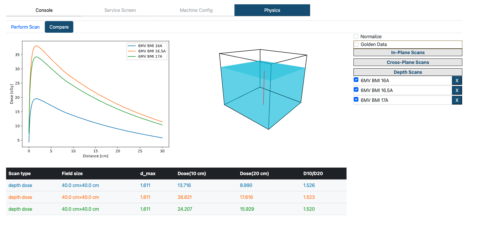
The Compare tab overlays multiple stored scans on a single plot, grouped by scan type, and can normalize them against golden beam data — the reference dataset for the beam model. A metrics table summarizes d_max, point doses and the D10/D20 ratio for each scan.
1
2
3
4
5
6
7
Numbered markers match the list below.
What each area does
1
Perform Scan / Compare tabs
Switch between running a new scan and comparing stored results.
2
Overlay plot
All selected scans drawn on one set of axes (here, depth-dose curves) for direct comparison.
3
Tank view
3-D view of the tank with the scan axis highlighted.
4
Normalize / Golden Data
Tick Golden Data and Normalize to compare your scans against the reference dataset on a common scale.
5
Scan groups
In-Plane, Cross-Plane and Depth Scans. Expand a group to list its stored scans.
6
Select / remove scans
Tick scans to overlay them; remove one from the list with its X button.
7
Metrics table
Per-scan summary: scan type, field size, d_max, Dose(10 cm), Dose(20 cm) and the D10/D20 ratio.
See also
Perform a scan
Calibration (TG51 / TRS-398)
Beam data / commissioning output
Physics Mode · Scanning Water Tank
Scanning Water Tank — compare scans
SCANNING WT · 2
The Compare tab overlays multiple stored scans on a single plot, grouped by scan type, and can normalize them against golden beam data — the reference dataset for the beam model. A metrics table summarizes d_max, point doses and the D10/D20 ratio for each scan.
1
2
3
4
5
6
7
Numbered markers match the list below.
What each area does
1
Perform Scan / Compare tabs
Switch between running a new scan and comparing stored results.
2
Overlay plot
All selected scans drawn on one set of axes (here, depth-dose curves) for direct comparison.
3
Tank view
3-D view of the tank with the scan axis highlighted.
4
Normalize / Golden Data
Tick Golden Data and Normalize to compare your scans against the reference dataset on a common scale.
5
Scan groups
In-Plane, Cross-Plane and Depth Scans. Expand a group to list its stored scans.
6
Select / remove scans
Tick scans to overlay them; remove one from the list with its X button.
7
Metrics table
Per-scan summary: scan type, field size, d_max, Dose(10 cm), Dose(20 cm) and the D10/D20 ratio.
See also
Perform a scan
Calibration (TG51 / TRS-398)
Beam data / commissioning output
Physics Mode · Calibrating Water Tank
Calibrating Water Tank — TG51 / TRS-398
CALIBRATING WT
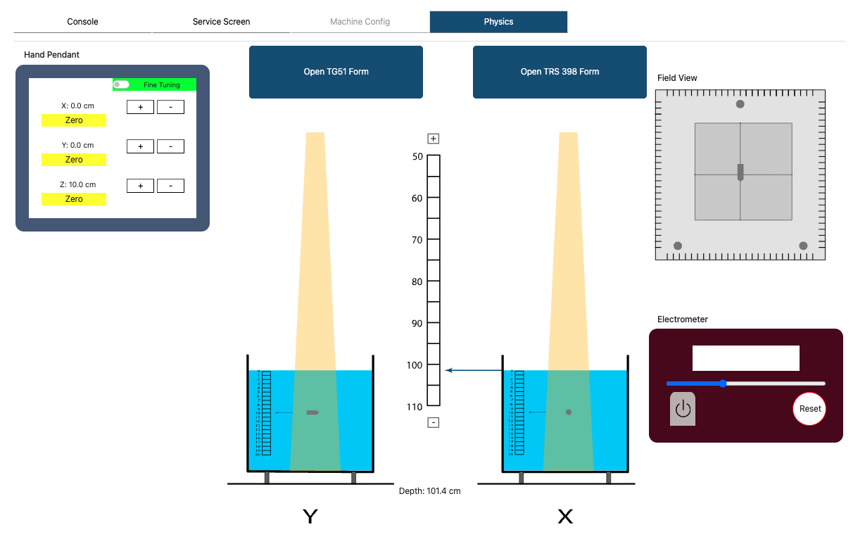
The second water tank is the Calibrating Water Tank. Instead of scanning profiles, it lets you work through a mock reference-dosimetry calibration — a TG51 or TRS-398 protocol — by positioning a chamber at depth, taking electrometer readings and entering them into the protocol form. Reach it from the Console (Physics Mode → Calibrating Water Tank).
1
2
3
4
5
6
7
8
Numbered markers match the list below.
Where next
Use this tank to practise an absolute-dose calibration end-to-end; use the Scanning Water Tank instead when you want beam profiles and depth-dose curves.
What each area does
1
Hand Pendant
Drive the chamber to an X / Y / Z position. Zero each axis, and toggle Fine Tuning for small steps.
2
Open TG51 Form
Opens the AAPM TG-51 absolute-dose calibration worksheet to enter your readings.
3
Open TRS 398 Form
Opens the IAEA TRS-398 calibration worksheet — the international counterpart to TG-51.
4
Depth ruler
Shared depth scale (with + / − nudge) tying the two tank views to a common depth; current depth is shown below.
5
Y tank view
Side view along Y showing the beam, water level and chamber depth.
6
X tank view
Side view along X — use the two views to centre the chamber on the beam axis.
7
Field View
Beam's-eye view of the field with the chamber position marked.
8
Electrometer
Reads the chamber signal; set the range, take a reading and Reset between measurements.
Step by step
1
Open the Calibrating Water Tank
From the Console choose Physics Mode then Calibrating Water Tank.
2
Position the chamber
Use the Hand Pendant to set X / Y / Z; centre on the beam using the X and Y tank views and the Field View, then set the calibration depth on the ruler.
3
Take readings
Turn on the beam and read the chamber signal on the electrometer; Reset between measurements.
4
Fill in the protocol
Open the TG51 or TRS-398 form and enter your readings and conditions to work through the calibration.
See also
Perform a scan
Beam data / commissioning output
Physics Mode · Calibrating Water Tank
Calibrating Water Tank — TG51 / TRS-398
CALIBRATING WT
The second water tank is the Calibrating Water Tank. Instead of scanning profiles, it lets you work through a mock reference-dosimetry calibration — a TG51 or TRS-398 protocol — by positioning a chamber at depth, taking electrometer readings and entering them into the protocol form. Reach it from the Console (Physics Mode → Calibrating Water Tank).
1
2
3
4
5
6
7
8
Numbered markers match the list below.
Where next
Use this tank to practise an absolute-dose calibration end-to-end; use the Scanning Water Tank instead when you want beam profiles and depth-dose curves.
What each area does
1
Hand Pendant
Drive the chamber to an X / Y / Z position. Zero each axis, and toggle Fine Tuning for small steps.
2
Open TG51 Form
Opens the AAPM TG-51 absolute-dose calibration worksheet to enter your readings.
3
Open TRS 398 Form
Opens the IAEA TRS-398 calibration worksheet — the international counterpart to TG-51.
4
Depth ruler
Shared depth scale (with + / − nudge) tying the two tank views to a common depth; current depth is shown below.
5
Y tank view
Side view along Y showing the beam, water level and chamber depth.
6
X tank view
Side view along X — use the two views to centre the chamber on the beam axis.
7
Field View
Beam's-eye view of the field with the chamber position marked.
8
Electrometer
Reads the chamber signal; set the range, take a reading and Reset between measurements.
Step by step
1
Open the Calibrating Water Tank
From the Console choose Physics Mode then Calibrating Water Tank.
2
Position the chamber
Use the Hand Pendant to set X / Y / Z; centre on the beam using the X and Y tank views and the Field View, then set the calibration depth on the ruler.
3
Take readings
Turn on the beam and read the chamber signal on the electrometer; Reset between measurements.
4
Fill in the protocol
Open the TG51 or TRS-398 form and enter your readings and conditions to work through the calibration.
See also
Perform a scan
Beam data / commissioning output
Service Mode
Service Mode
SERVICE MODE VARIAN
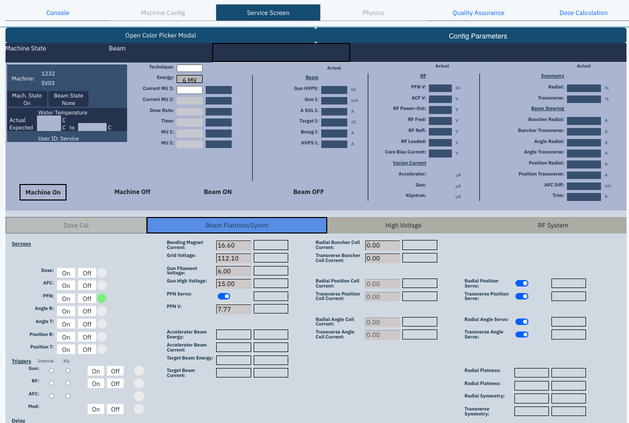
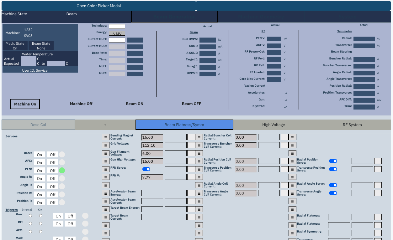
The Service Screen is a copy of Machine Config presented in an interface that matches a real Varian service screen. Changes made in either screen are reflected in the other, so you can set your machine parameters here and investigate the outputs exactly as you would in Machine Config.
Getting there
Select a machine and Service Mode, then open the Service Screen tab. You land on your default screen. These screens are fully configurable — colours, parameter names, parameter order and the tabs themselves.
1
2
3
4
5
6
7
The default Varian service screen. On Varian the profile plots sit below the screen. Numbered markers match the list below.
1
Service Screen tab
Opens Service Mode for the machine you selected.
2
Open Color Picker Modal
Opens the Color Customization pop-up.
3
Config Parameters
Switches the screen into edit mode.
4
Machine State
Machine and beam state, water temperature and user ID.
5
Set and Actual columns
The value you asked for beside the value the machine is producing.
6
Machine and beam controls
Machine On and Off, Beam ON and OFF.
7
Parameter group tabs
Dose Cal, Beam Flatness/Symm, High Voltage and RF System.
Matching your colours
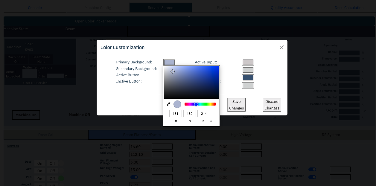
Selecting Open Color Picker Modal brings up the Color Customization pop-up, where you set the primary and secondary backgrounds, the active and inactive inputs and the active and inactive buttons. Save Changes applies them; Discard Changes backs out.
Primary background#b5bdd6
Secondary background#d6dee6
Common Varian values.
The Color Customization pop-up, with a picker for each element of the interface.
Rearranging parameters
Selecting Config Parameters switches the screen into edit mode.
1
Move a parameter
Drag and drop it into place using the three-lined icon to the left of the parameter.
2
Add a parameter
Select the + button within a tab and choose from the available Machine Config parameters.
3
Add a tab
The + button at the tabs adds another tab. Name it, then populate it with parameters.
4
Rename a parameter
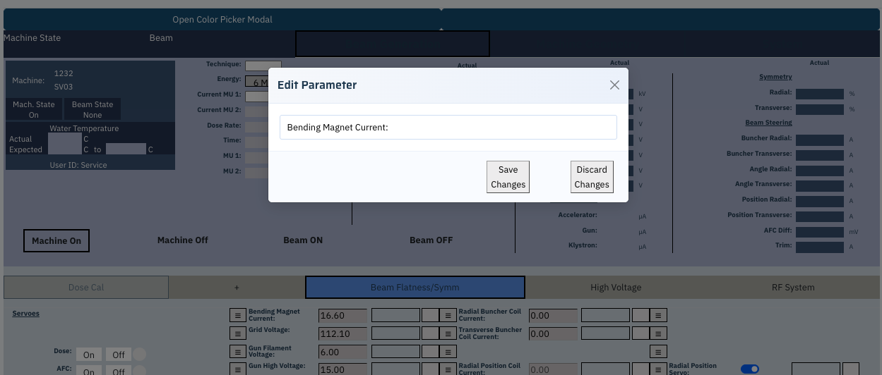
Click the edit icon to the right of the parameter. A pop-up appears where you change the name and save it.
1
2
3
4
Edit mode — every parameter gains a drag handle and an edit icon, and the tabs gain a + button. Numbered markers match the list below.
1
Open Color Picker Modal
Stays available while you are in edit mode.
2
Drag handle
The three-lined icon to the left of a parameter — drag it to move the parameter.
3
Edit icon
To the right of a parameter — opens the rename pop-up.
4
Add a tab
The + button at the tabs adds another tab for you to name and populate.
The Edit Parameter pop-up, reached from the edit icon beside a parameter.
Reading the outputs
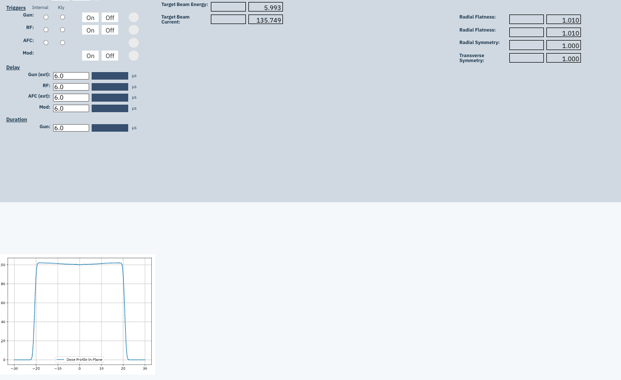
On Varian the profile plots sit below the screen. Set values sit beside actual values throughout, so you can compare what you asked the machine for against what it is producing.
A beam running on the Varian service screen, with its profile plots and readouts.
See also
Screen layout
Overview
Servos
Service Mode
Service Mode
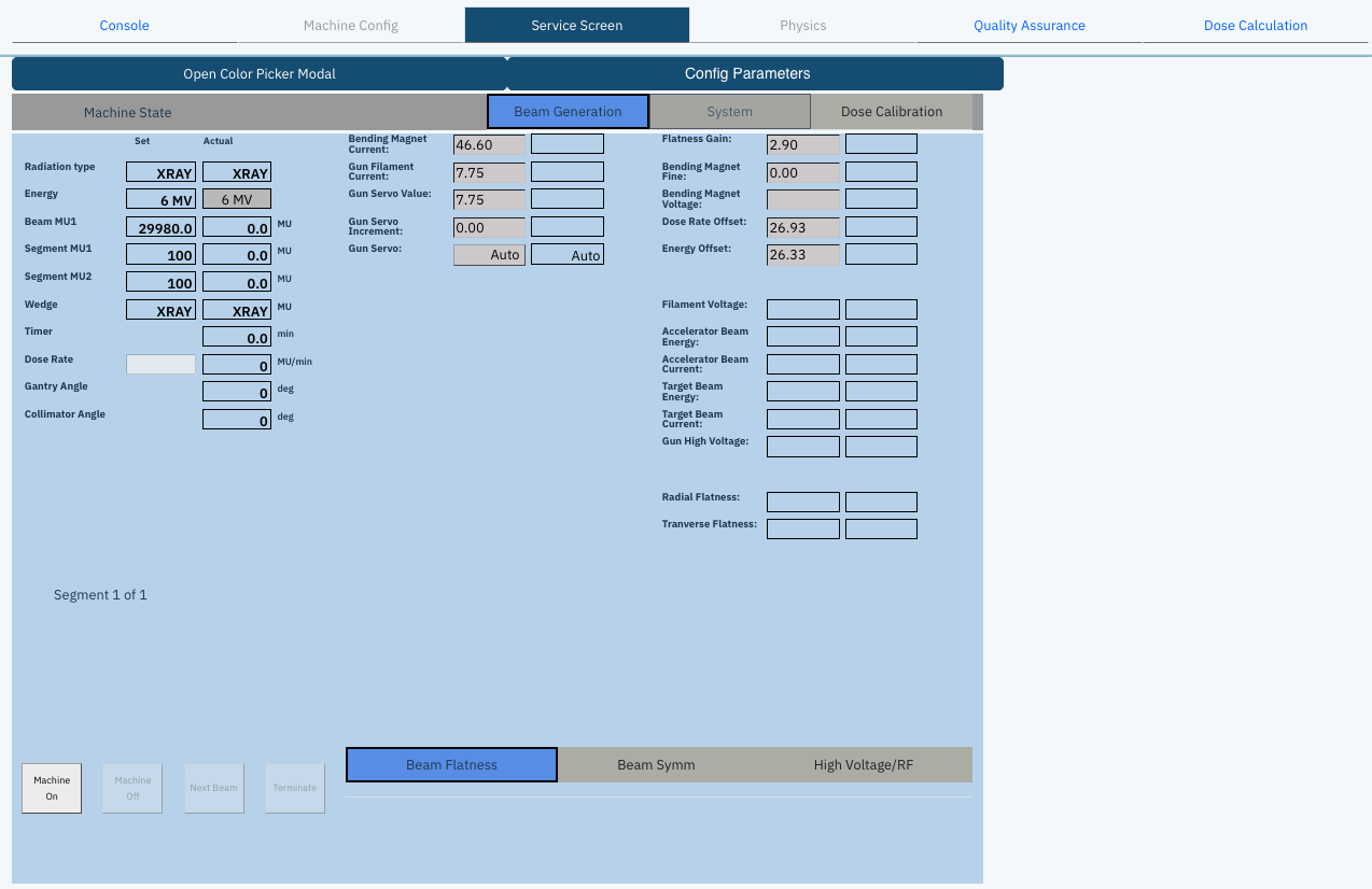
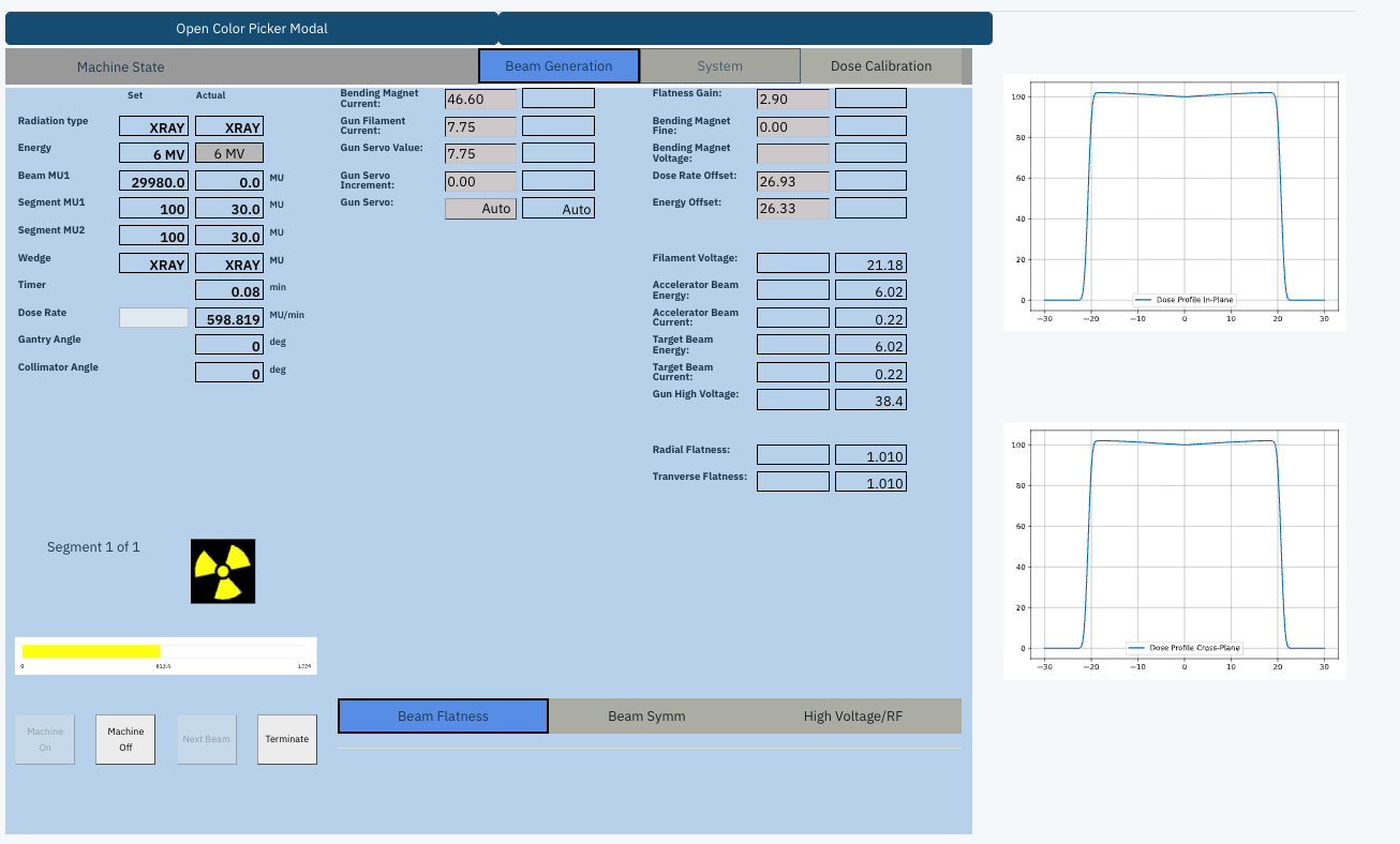
SERVICE MODE ELEKTA
The Service Screen is a copy of Machine Config presented in an interface that matches a real Elekta service screen. Changes made in either screen are reflected in the other, so you can set your machine parameters here and investigate the outputs exactly as you would in Machine Config.
Getting there
Select a machine and Service Mode, then open the Service Screen tab. You land on your default screen. These screens are fully configurable — colours, parameter names, parameter order and the tabs themselves.
1
2
3
4
5
6
7
The default Elekta service screen. On Elekta the profile plots sit to the right of the screen. Numbered markers match the list below.
1
Service Screen tab
Opens Service Mode for the machine you selected.
2
Open Color Picker Modal
Opens the Color Customization pop-up.
3
Config Parameters
Switches the screen into edit mode.
4
Parameter group tabs
Machine State, Beam Generation, System and Dose Calibration.
5
Set and Actual columns
The value you asked for beside the value the machine is producing.
6
Beam group tabs
Beam Flatness, Beam Symm and High Voltage/RF.
7
Machine and beam controls
Machine On and Off, Next Beam and Terminate.
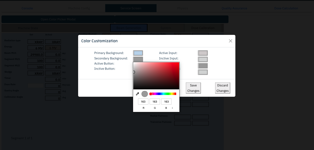
Matching your colours
Selecting Open Color Picker Modal brings up the Color Customization pop-up, where you set the primary and secondary backgrounds, the active and inactive inputs and the active and inactive buttons. Save Changes applies them; Discard Changes backs out.
Primary background#c0d3cf
Common Elekta values.
The Color Customization pop-up, with a picker for each element of the interface.
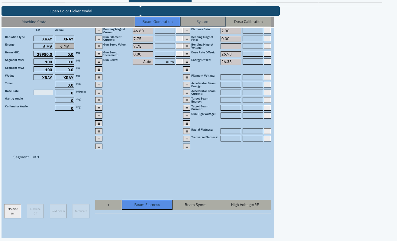
Rearranging parameters
Selecting Config Parameters switches the screen into edit mode.
1
Move a parameter
Drag and drop it into place using the three-lined icon to the left of the parameter.
2
Add a parameter
Select the + button within a tab and choose from the available Machine Config parameters.
3
Add a tab
The + button at the tabs adds another tab. Name it, then populate it with parameters.
4
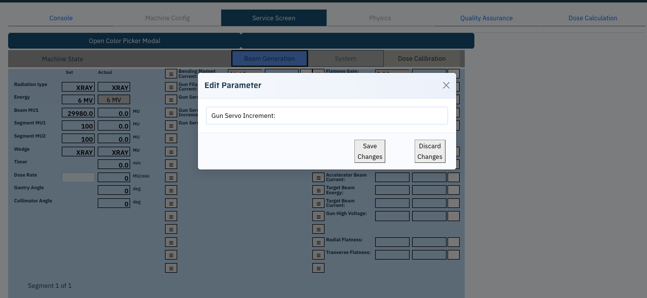
Rename a parameter
Click the edit icon to the right of the parameter. A pop-up appears where you change the name and save it.
1
2
3
4
Edit mode — every parameter gains a drag handle and an edit icon, and the tabs gain a + button. Numbered markers match the list below.
1
Open Color Picker Modal
Stays available while you are in edit mode.
2
Drag handle
The three-lined icon to the left of a parameter — drag it to move the parameter.
3
Edit icon
To the right of a parameter — opens the rename pop-up.
4
Add a tab
The + button at the tabs adds another tab for you to name and populate.
The Edit Parameter pop-up, reached from the edit icon beside a parameter.
Reading the outputs
On Elekta the profile plots sit to the right of the screen. Set values sit beside actual values throughout, so you can compare what you asked the machine for against what it is producing.
A beam running on the Elekta service screen, with its profile plots and readouts.
See also
Screen layout
Overview
Servos
Quality Assurance
SIMAC QA
QUALITY ASSURANCE
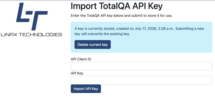
Import your real QA data from TotalQA by Image Owl. Connect with an API key to reach every report across your machines and sites, then overlay a measured plot onto the simulator in Machine Config to match your beam model virtually.
1 · Link your TotalQA account
In the username drop-down in the top-right corner, navigate to TotalQA API Keys and enter the API key found in your TotalQA account. This links your data.
If a key is already stored, submitting a new one overwrites it. Use Delete current key to clear it instead.
Enter the API Client ID and API Key, then Import API Key.
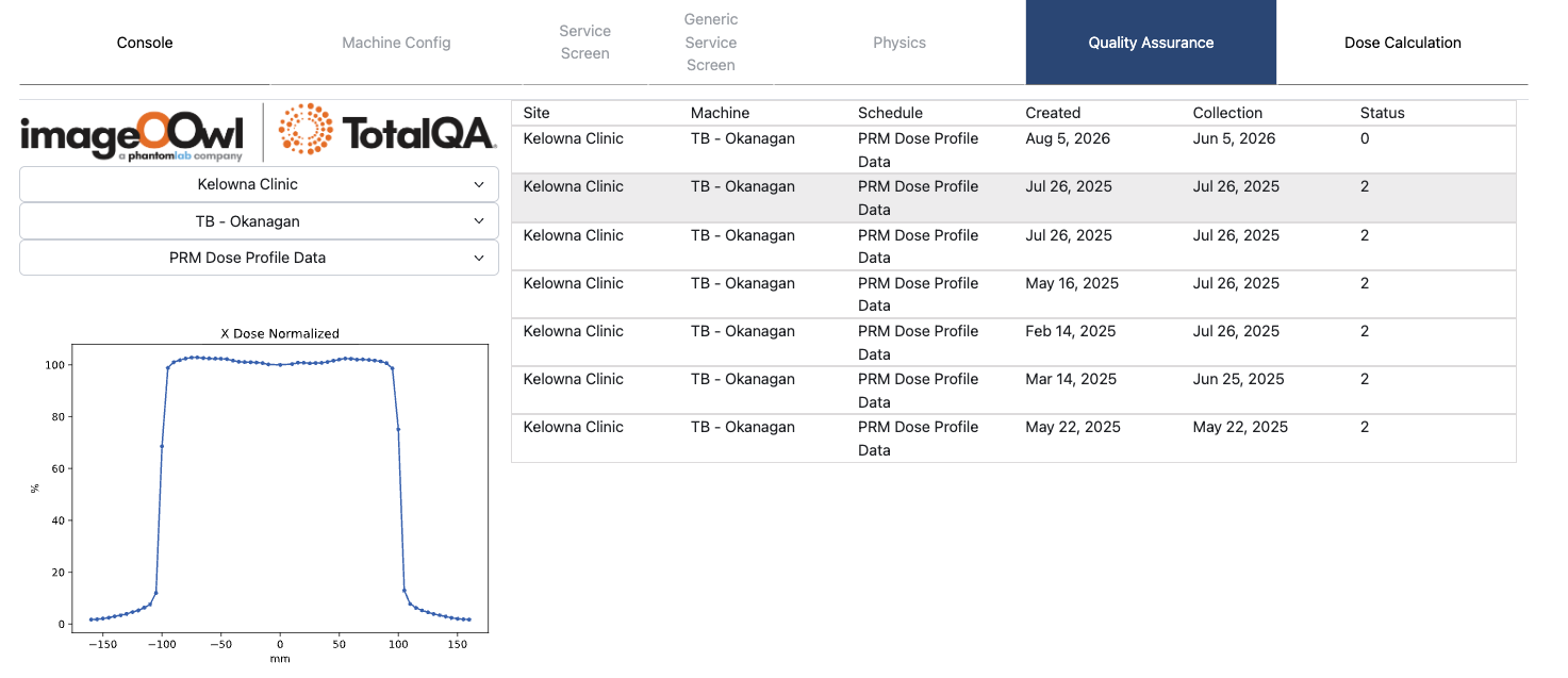
2 · Find your reports
The three drop-downs select site, machine and schedule to populate your QA reports exactly as they appear in TotalQA.
1
2
3
4
1
Site, machine & schedule
The three drop-downs that filter which reports are listed.
2
Report list
Every matching report with its created and collection dates, and status.
3
Status
How many results the collection holds.
4
Plot
The selected report drawn out — this is the plot that becomes available to overlay.
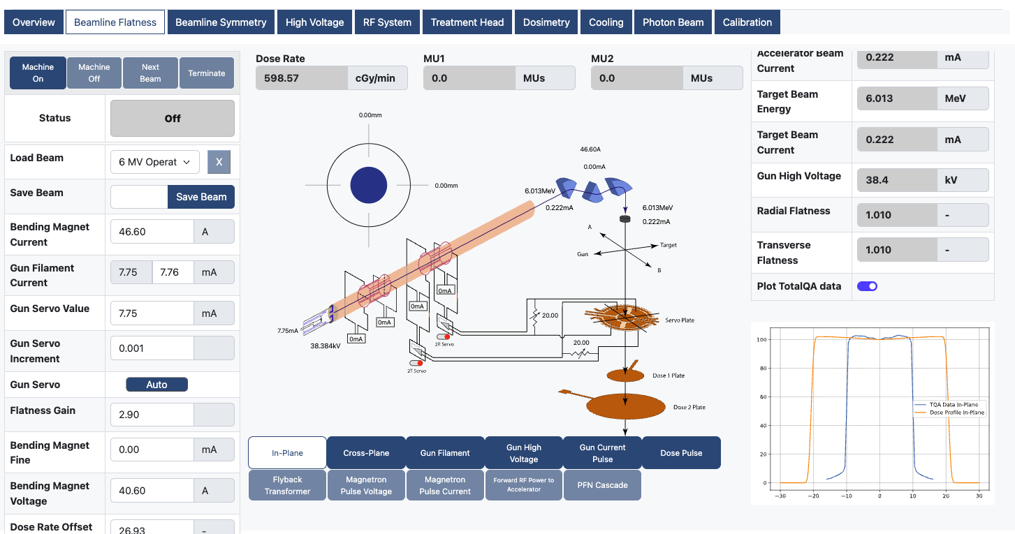
3 · Overlay it in Machine Config
Whichever report is selected and has its plot visible becomes available to overlay on your plots in Machine Config.
Switch to Machine Config and turn on Plot TotalQA data. Your measured curve is drawn against the simulated one, so you can tune inputs until the model matches the machine.
Plot TotalQA data toggled on — measured data overlaid on the simulated profile.
See also
Beamline Flatness
Perform a scan
Beam data / commissioning output
Quality Assurance
SIMAC QA
QUALITY ASSURANCE
Import your real QA data from TotalQA by Image Owl. Connect with an API key to reach every report across your machines and sites, then overlay a measured plot onto the simulator in Machine Config to match your beam model virtually.
1 · Link your TotalQA account
In the username drop-down in the top-right corner, navigate to TotalQA API Keys and enter the API key found in your TotalQA account. This links your data.
If a key is already stored, submitting a new one overwrites it. Use Delete current key to clear it instead.
Enter the API Client ID and API Key, then Import API Key.
2 · Find your reports
The three drop-downs select site, machine and schedule to populate your QA reports exactly as they appear in TotalQA.
1
2
3
4
1
Site, machine & schedule
The three drop-downs that filter which reports are listed.
2
Report list
Every matching report with its created and collection dates, and status.
3
Status
How many results the collection holds.
4
Plot
The selected report drawn out — this is the plot that becomes available to overlay.
3 · Overlay it in Machine Config
Whichever report is selected and has its plot visible becomes available to overlay on your plots in Machine Config.
Switch to Machine Config and turn on Plot TotalQA data. Your measured curve is drawn against the simulated one, so you can tune inputs until the model matches the machine.
Plot TotalQA data toggled on — measured data overlaid on the simulated profile.
See also
Beamline Flatness
Perform a scan
Beam data / commissioning output
Dose Calculation
SIMAC Dose Calc
DOSE CALCULATION
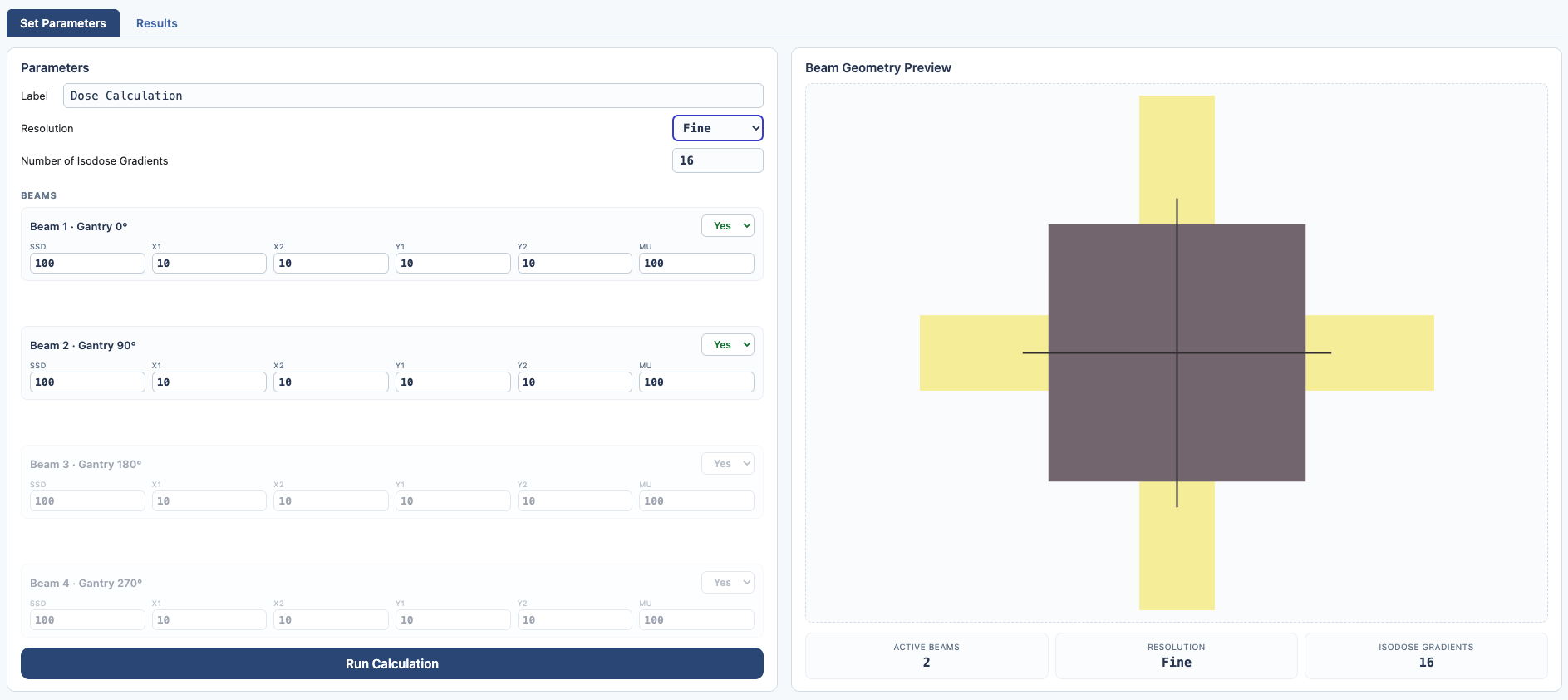
Perform a four-field dose calculation to investigate dose distributions. Set up the calculation on the Set Parameters tab, run it, then read the resulting multi-field distribution on the Results tab.
Set Parameters
1
2
3
4
5
6
1
Label
Name the calculation so you can find it on the Results tab.
2
Resolution & isodose gradients
Set the calculation resolution and the number of isodose gradients drawn on the plot.
3
Beams
Four gantry angles — 0°, 90°, 180° and 270°. Set Yes or No on each to choose which fields are delivered.
4
Per-beam settings
For each field: SSD, jaw positions (X1/X2, Y1/Y2) and the MUs to deliver.
5
Run Calculation
Runs the multi-field calculation and stores it under your label.
6
Beam geometry preview
A live view of the fields you have enabled, with active beams, resolution and gradients summarised underneath.
Step by step
1
Open the Dose Calc tab
Navigating to the Dose Calc tab lands on the Set Parameters tab, where you set up the calculation.
2
Name and configure
Give it a label, set the resolution and the number of isodose gradients.
3
Choose the beam and fields
Select a saved beam and which of the four fields you would like to deliver.
4
Set the delivery
Finally set the SSD, field size and MUs to deliver for each active field.
5
Calculate
Select Calculate Dose Multi Field, then navigate to Results to see the distribution.
Results
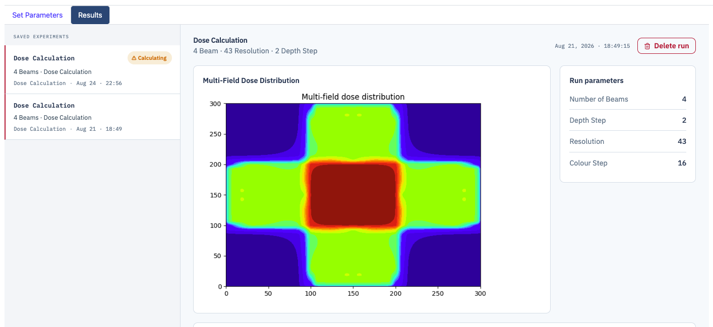
The Results tab lists calculated and already-calculated beams. Clicking a result shows its dose distribution plot alongside the set-up parameters it was run with.
Delete Run removes the scan from the Results tab. This is not reversible.
A multi-field dose distribution with its run parameters on the right.
See also
Treatment Head
Perform a scan
Dose Calculation
SIMAC Dose Calc
DOSE CALCULATION
Perform a four-field dose calculation to investigate dose distributions. Set up the calculation on the Set Parameters tab, run it, then read the resulting multi-field distribution on the Results tab.
Set Parameters
1
2
3
4
5
6
1
Label
Name the calculation so you can find it on the Results tab.
2
Resolution & isodose gradients
Set the calculation resolution and the number of isodose gradients drawn on the plot.
3
Beams
Four gantry angles — 0°, 90°, 180° and 270°. Set Yes or No on each to choose which fields are delivered.
4
Per-beam settings
For each field: SSD, jaw positions (X1/X2, Y1/Y2) and the MUs to deliver.
5
Run Calculation
Runs the multi-field calculation and stores it under your label.
6
Beam geometry preview
A live view of the fields you have enabled, with active beams, resolution and gradients summarised underneath.
Step by step
1
Open the Dose Calc tab
Navigating to the Dose Calc tab lands on the Set Parameters tab, where you set up the calculation.
2
Name and configure
Give it a label, set the resolution and the number of isodose gradients.
3
Choose the beam and fields
Select a saved beam and which of the four fields you would like to deliver.
4
Set the delivery
Finally set the SSD, field size and MUs to deliver for each active field.
5
Calculate
Select Calculate Dose Multi Field, then navigate to Results to see the distribution.
Results
The Results tab lists calculated and already-calculated beams. Clicking a result shows its dose distribution plot alongside the set-up parameters it was run with.
Delete Run removes the scan from the Results tab. This is not reversible.
A multi-field dose distribution with its run parameters on the right.
See also
Treatment Head
Perform a scan
How-to guide
Read & interpret outputs
Dose rate, beam energy, flatness, symmetry
GUIDE 02
Goal
Understand what each live readout means and what "good" looks like before you start tuning.
1
Dose Rate, MU1, MU2
Always present. Dose Rate is the physical output at the measurement point; MU1 and MU2 are the two independent monitor-chamber channels and should track each other.
2
Flatness
Radial and Transverse Flatness describe how uniform the profile is across the field. Reported on Overview and Beamline tabs.
Beamline Flatness →
3
Symmetry
Radial and Transverse Symmetry are point-difference values (100 × max difference of mirrored points). Closer to 0 % is better.
4
RF tuning signals
On the RF tab, Tuner Drive and Phase Error show how hard the AFC servo is working to stay on resonance.
RF System →
5
Investigate waveforms
Use the plot selector to see how our beam state effects various relationships including Flatness, Symmetry, Reflected pulse, and more.
Tips
Compare MU1 and MU2: a divergence between channels points to a dosimetry or monitor-chamber issue, not a beam-generation one.
Flatness and symmetry are evaluated on the profile — plot In-Plane and Cross-Plane to see the shape behind the numbers.
Related tabs
Dosimetry
Beamline Flatness
RF System
How-to guide
Read & interpret outputs
Dose rate, beam energy, flatness, symmetry
GUIDE 02
Goal
Understand what each live readout means and what "good" looks like before you start tuning.
1
Dose Rate, MU1, MU2
Always present. Dose Rate is the physical output at the measurement point; MU1 and MU2 are the two independent monitor-chamber channels and should track each other.
2
Flatness
Radial and Transverse Flatness describe how uniform the profile is across the field. Reported on Overview and Beamline tabs.
Beamline Flatness →
3
Symmetry
Radial and Transverse Symmetry are point-difference values (100 × max difference of mirrored points). Closer to 0 % is better.
4
RF tuning signals
On the RF tab, Tuner Drive and Phase Error show how hard the AFC servo is working to stay on resonance.
RF System →
5
Investigate waveforms
Use the plot selector to see how our beam state effects various relationships including Flatness, Symmetry, Reflected pulse, and more.
Tips
Compare MU1 and MU2: a divergence between channels points to a dosimetry or monitor-chamber issue, not a beam-generation one.
Flatness and symmetry are evaluated on the profile — plot In-Plane and Cross-Plane to see the shape behind the numbers.
Related tabs
Dosimetry
Beamline Flatness
RF System
How-to guide
Tune flatness & symmetry
Which inputs move them, and the cause & effect
GUIDE 03
Goal
Bring radial/transverse flatness and symmetry into tolerance using the steering, bending-magnet and energy inputs.
1
Start from symmetry
Symmetry responds to beam steering. The gun-end coils (Buncher / 1-series) are the most sensitive; the mid-guide coils (Position / 2-series) are less so.
Beamline Symmetry →
2
Steer radial vs transverse separately
Radial coils move the gun–target axis; transverse coils move left–right. Adjust the matching pair for the axis that is off.
3
Let servos hold it
Enable the angle/position servos (Varian) or 2R/2T servos (Elekta) to drive the coils automatically once you are close.
4
Then flatness
Flatness tracks energy on the target and the flattening filter. Trim the Bending Magnet Current and Beam STD; the Flatness Gain / hump balance compares inner vs outer chamber segments.
5
Re-check the other axis
Steering changes interact — after fixing one axis, re-read both symmetry values and iterate.
Tips
Make one change at a time and watch a single output; the loops interact and ganged changes are hard to unwind.
If symmetry will not settle, check gun error first — a misaligned gun biases every downstream correction.
Related tabs
Beamline Flatness
Overview
Dosimetry
How-to guide
Tune flatness & symmetry
Which inputs move them, and the cause & effect
GUIDE 03
Goal
Bring radial/transverse flatness and symmetry into tolerance using the steering, bending-magnet and energy inputs.
1
Start from symmetry
Symmetry responds to beam steering. The gun-end coils (Buncher / 1-series) are the most sensitive; the mid-guide coils (Position / 2-series) are less so.
Beamline Symmetry →
2
Steer radial vs transverse separately
Radial coils move the gun–target axis; transverse coils move left–right. Adjust the matching pair for the axis that is off.
3
Let servos hold it
Enable the angle/position servos (Varian) or 2R/2T servos (Elekta) to drive the coils automatically once you are close.
4
Then flatness
Flatness tracks energy on the target and the flattening filter. Trim the Bending Magnet Current and Beam STD; the Flatness Gain / hump balance compares inner vs outer chamber segments.
5
Re-check the other axis
Steering changes interact — after fixing one axis, re-read both symmetry values and iterate.
Tips
Make one change at a time and watch a single output; the loops interact and ganged changes are hard to unwind.
If symmetry will not settle, check gun error first — a misaligned gun biases every downstream correction.
Related tabs
Beamline Flatness
Overview
Dosimetry
How-to guide
Explore energy
How target, bending magnet & beam energy shape depth dose and profiles
GUIDE 04
Goal
See how the energy-selecting chain changes percentage depth dose (PDD) and off-axis profiles.
1
Select energy at the bending magnet
Bending Magnet Current sets which electron energy follows the correct radius through the magnet; the energy slit trims the spread.
Beamline Flatness →
2
Set the spectrum width
Beam STD widens or narrows the Gaussian energy spread — affecting penetration and profile shape.
3
Change the target
Target material and thickness change bremsstrahlung production and hardening. Re-optimize the filter afterward.
Treatment Head →
4
Compare PDD
Plot the depth-dose curve and watch how higher effective energy pushes Dmax deeper and raises exit dose.
5
Watch flatness shift
Energy changes alter off-axis softening — expect to re-tune flatness after any significant energy move.
Tips
Energy, target and filter are coupled — change one and the flat-profile assumption behind the filter no longer holds.
Use the Optimize Filter action (Varian) after changing energy or target to restore a flat profile.
Related tabs
Beamline Flatness
Treatment Head
RF System
How-to guide
Explore energy
How target, bending magnet & beam energy shape depth dose and profiles
GUIDE 04
Goal
See how the energy-selecting chain changes percentage depth dose (PDD) and off-axis profiles.
1
Select energy at the bending magnet
Bending Magnet Current sets which electron energy follows the correct radius through the magnet; the energy slit trims the spread.
Beamline Flatness →
2
Set the spectrum width
Beam STD widens or narrows the Gaussian energy spread — affecting penetration and profile shape.
3
Change the target
Target material and thickness change bremsstrahlung production and hardening. Re-optimize the filter afterward.
Treatment Head →
4
Compare PDD
Plot the depth-dose curve and watch how higher effective energy pushes Dmax deeper and raises exit dose.
5
Watch flatness shift
Energy changes alter off-axis softening — expect to re-tune flatness after any significant energy move.
Tips
Energy, target and filter are coupled — change one and the flat-profile assumption behind the filter no longer holds.
Use the Optimize Filter action (Varian) after changing energy or target to restore a flat profile.
Related tabs
Beamline Flatness
Treatment Head
RF System
How-to guide
Beam data / commissioning output
The hand-off to Simac Water Tank
GUIDE 06
Goal
Produce commissioning-style beam data from a tuned beam and pass it to the virtual Water Tank.
1
Tune and lock the beam
Get flatness, symmetry and output in tolerance, then Save Beam so the operating point is fixed.
2
Set scan conditions
Confirm SSD and field size on the Treatment Head tab to match your commissioning protocol.
Treatment Head →
3
Collect profiles & depth dose
Use the profile/scan tools to capture cross-plane, in-plane and depth-dose curves at the required depths.
4
Hand off to Water Tank
Switch to Physics Mode (or the Physics tab) and select the saved beam in the Water Tank to run In-Plane, Cross-Plane and Depth scans, then compare against golden data.
Perform a scan →
Tips
Commissioning data is only as good as the locked operating point — re-verify outputs immediately before collecting.
Keep SSD and field size consistent with the protocol you will validate against.
Related tabs
Perform a scan
Compare scans
Treatment Head
Dosimetry
How-to guide
Beam data / commissioning output
The hand-off to Simac Water Tank
GUIDE 06
Goal
Produce commissioning-style beam data from a tuned beam and pass it to the virtual Water Tank.
1
Tune and lock the beam
Get flatness, symmetry and output in tolerance, then Save Beam so the operating point is fixed.
2
Set scan conditions
Confirm SSD and field size on the Treatment Head tab to match your commissioning protocol.
Treatment Head →
3
Collect profiles & depth dose
Use the profile/scan tools to capture cross-plane, in-plane and depth-dose curves at the required depths.
4
Hand off to Water Tank
Switch to Physics Mode (or the Physics tab) and select the saved beam in the Water Tank to run In-Plane, Cross-Plane and Depth scans, then compare against golden data.
Perform a scan →
Tips
Commissioning data is only as good as the locked operating point — re-verify outputs immediately before collecting.
Keep SSD and field size consistent with the protocol you will validate against.
Related tabs
Perform a scan
Compare scans
Treatment Head
Dosimetry
How-to guide
Troubleshoot
Symptom → likely subsystem → parameter
GUIDE 07
Goal
Move from an out-of-tolerance readout to the subsystem and input most likely responsible.